6 Analysis of metastatic disease profiles
I proceed with the multivariate analysis of the metastatic disease profiles between dnMBC and rMBC. We agreed that we characterize the differences only for the more recent cases, at least 2015. You will see the original analysis performed on the whole cohort (from 2000) and then a secondary analysis on the sub-cohort from 2015. We will first characterize the prevalence of the single sites and then of the co-occurrence.
For the co-occurrence we then proceed to a multivariate analysis: multiple correspondence analysis and hierarchical clustering on principal components.
6.0.1 Relative frequencies of site occurrence
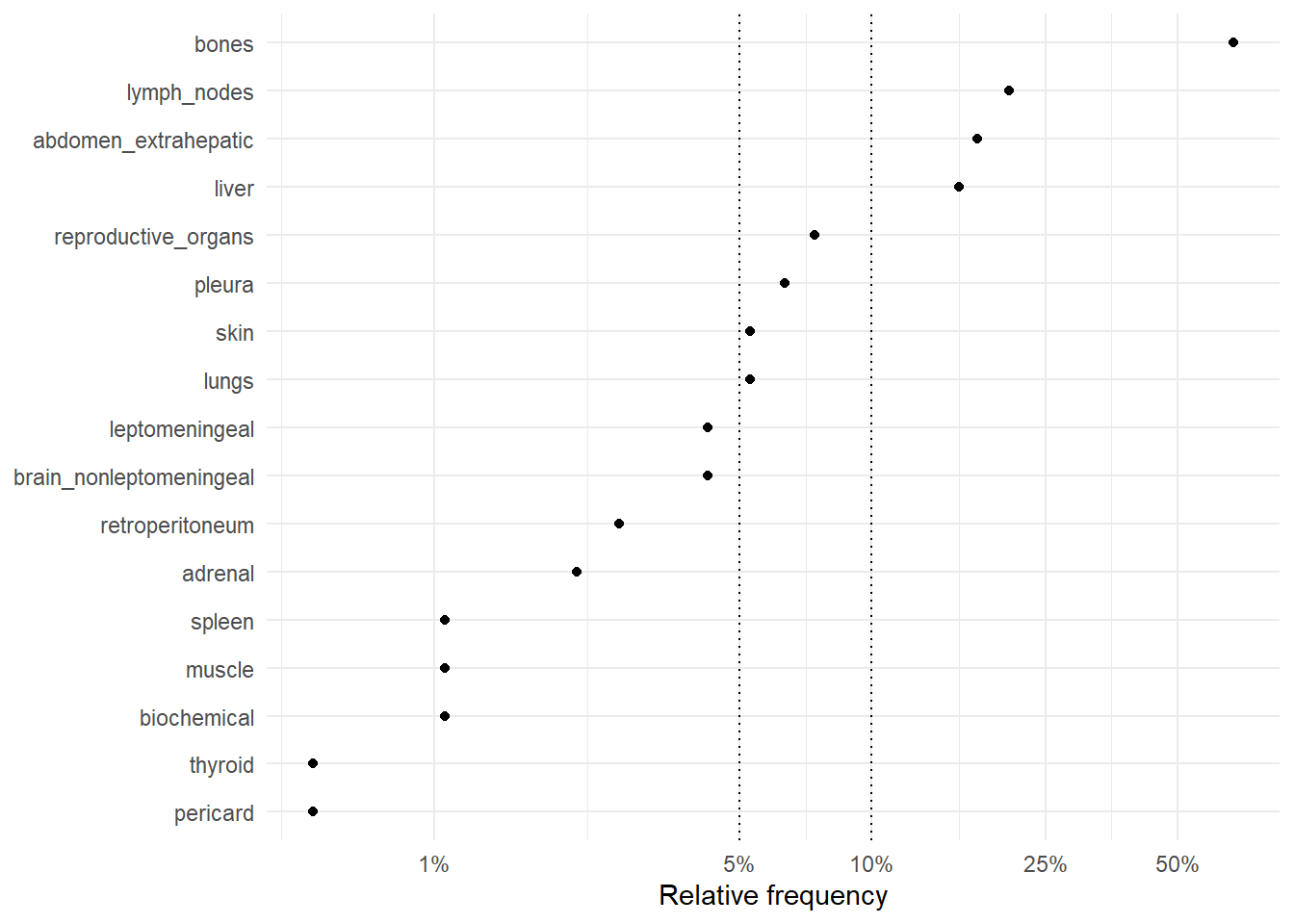
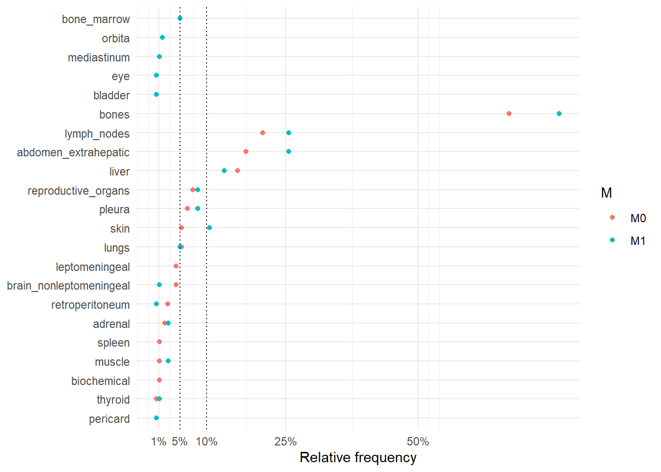
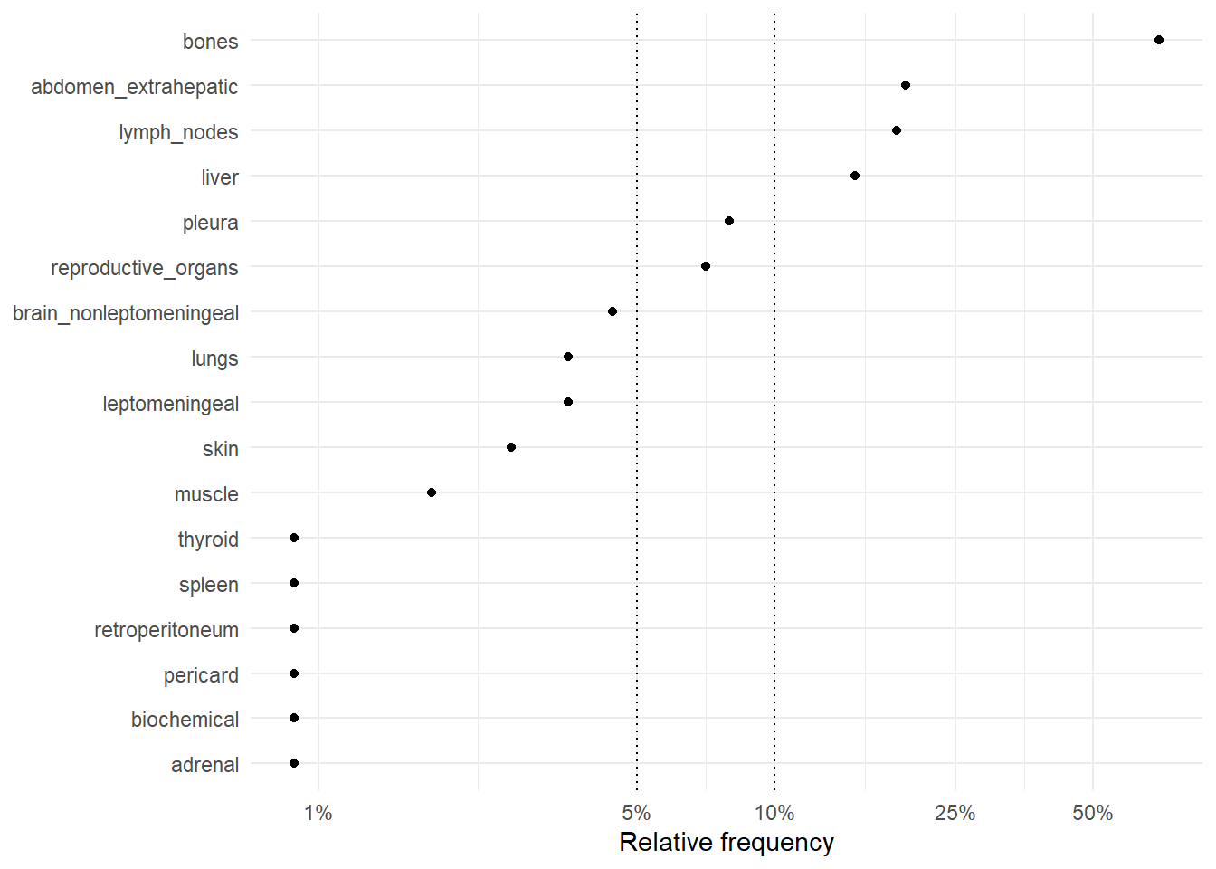
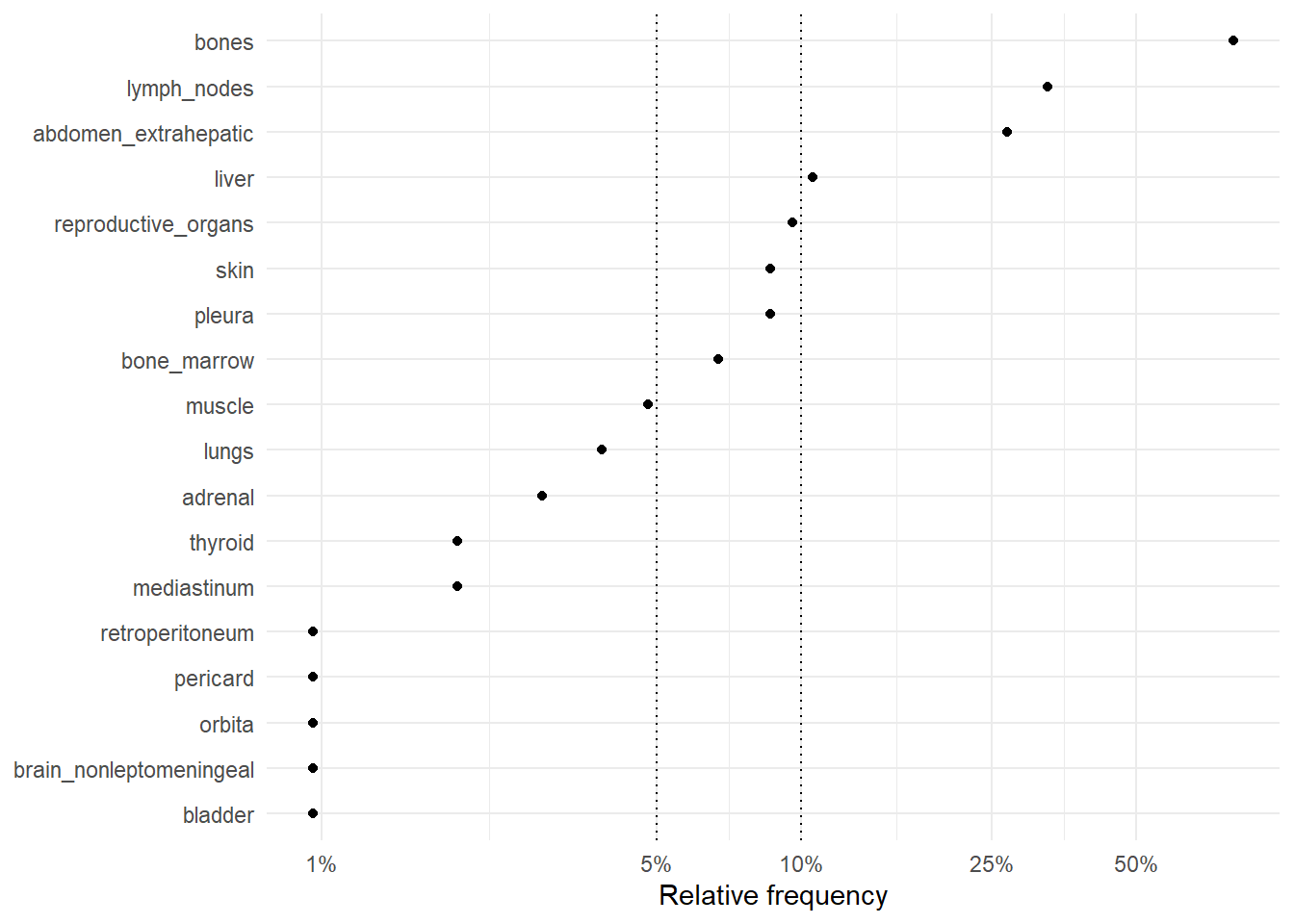
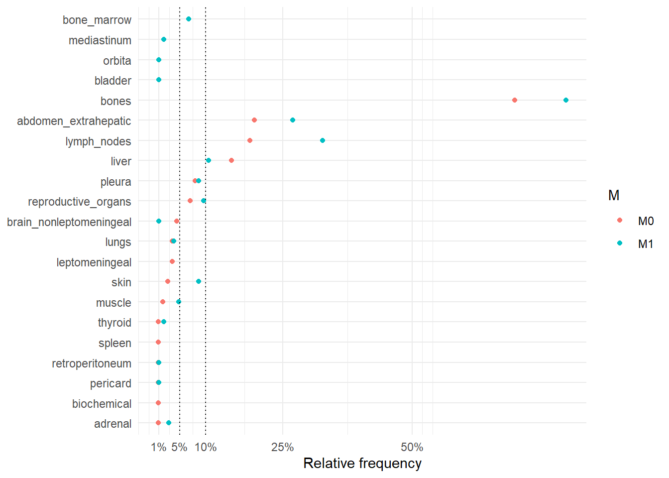
The following figures represent the relative frequencies of occurrence of each site for rM0 and dnM1 patients.
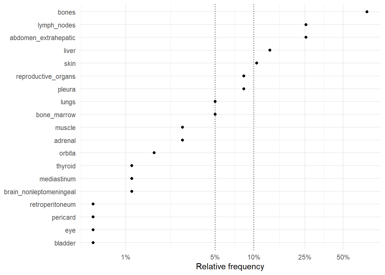
The following figure represents the comparison of the occurrence sites between rM0 and dnM1.
The following table summarize the differences between rM0 and dnM1 in terms of number of sites involved in the metastatic disease and the individual site where metastases occurred.
| M0 (N=189) |
M1 (N=180) |
Overall (N=369) |
|
|---|---|---|---|
| Number of sites | |||
| 1 | 111 (58.7%) | 86 (47.8%) | 197 (53.4%) |
| 2 | 48 (25.4%) | 48 (26.7%) | 96 (26.0%) |
| 3 | 20 (10.6%) | 30 (16.7%) | 50 (13.6%) |
| 4 | 9 (4.8%) | 12 (6.7%) | 21 (5.7%) |
| 5 | 1 (0.5%) | 2 (1.1%) | 3 (0.8%) |
| 8 | 0 (0%) | 1 (0.6%) | 1 (0.3%) |
| 6 | 0 (0%) | 1 (0.6%) | 1 (0.3%) |
| bones | |||
| no | 62 (32.8%) | 42 (23.3%) | 104 (28.2%) |
| yes | 127 (67.2%) | 138 (76.7%) | 265 (71.8%) |
| abdomen_extrahepatic | |||
| no | 156 (82.5%) | 134 (74.4%) | 290 (78.6%) |
| yes | 33 (17.5%) | 46 (25.6%) | 79 (21.4%) |
| liver | |||
| no | 159 (84.1%) | 156 (86.7%) | 315 (85.4%) |
| yes | 30 (15.9%) | 24 (13.3%) | 54 (14.6%) |
| lymph_nodes | |||
| no | 150 (79.4%) | 134 (74.4%) | 284 (77.0%) |
| yes | 39 (20.6%) | 46 (25.6%) | 85 (23.0%) |
| pleura | |||
| no | 177 (93.7%) | 165 (91.7%) | 342 (92.7%) |
| yes | 12 (6.3%) | 15 (8.3%) | 27 (7.3%) |
| reproductive_organs | |||
| no | 175 (92.6%) | 165 (91.7%) | 340 (92.1%) |
| yes | 14 (7.4%) | 15 (8.3%) | 29 (7.9%) |
| brain_nonleptomeningeal | |||
| no | 181 (95.8%) | 178 (98.9%) | 359 (97.3%) |
| yes | 8 (4.2%) | 2 (1.1%) | 10 (2.7%) |
| lungs | |||
| no | 179 (94.7%) | 171 (95.0%) | 350 (94.9%) |
| yes | 10 (5.3%) | 9 (5.0%) | 19 (5.1%) |
| leptomeningeal | |||
| no | 181 (95.8%) | 180 (100%) | 361 (97.8%) |
| yes | 8 (4.2%) | 0 (0%) | 8 (2.2%) |
| pericard | |||
| no | 188 (99.5%) | 179 (99.4%) | 367 (99.5%) |
| yes | 1 (0.5%) | 1 (0.6%) | 2 (0.5%) |
| skin | |||
| no | 179 (94.7%) | 161 (89.4%) | 340 (92.1%) |
| yes | 10 (5.3%) | 19 (10.6%) | 29 (7.9%) |
| spleen | |||
| no | 187 (98.9%) | 180 (100%) | 367 (99.5%) |
| yes | 2 (1.1%) | 0 (0%) | 2 (0.5%) |
| retroperitoneum | |||
| no | 184 (97.4%) | 179 (99.4%) | 363 (98.4%) |
| yes | 5 (2.6%) | 1 (0.6%) | 6 (1.6%) |
| adrenal | |||
| no | 185 (97.9%) | 175 (97.2%) | 360 (97.6%) |
| yes | 4 (2.1%) | 5 (2.8%) | 9 (2.4%) |
| muscle | |||
| no | 187 (98.9%) | 175 (97.2%) | 362 (98.1%) |
| yes | 2 (1.1%) | 5 (2.8%) | 7 (1.9%) |
| biochemical | |||
| no | 187 (98.9%) | 180 (100%) | 367 (99.5%) |
| yes | 2 (1.1%) | 0 (0%) | 2 (0.5%) |
| thyroid | |||
| no | 188 (99.5%) | 178 (98.9%) | 366 (99.2%) |
| yes | 1 (0.5%) | 2 (1.1%) | 3 (0.8%) |
| orbita | |||
| no | 189 (100%) | 177 (98.3%) | 366 (99.2%) |
| yes | 0 (0%) | 3 (1.7%) | 3 (0.8%) |
| eye | |||
| no | 189 (100%) | 179 (99.4%) | 368 (99.7%) |
| yes | 0 (0%) | 1 (0.6%) | 1 (0.3%) |
| bone_marrow | |||
| no | 189 (100%) | 171 (95.0%) | 360 (97.6%) |
| yes | 0 (0%) | 9 (5.0%) | 9 (2.4%) |
| bladder | |||
| no | 189 (100%) | 179 (99.4%) | 368 (99.7%) |
| yes | 0 (0%) | 1 (0.6%) | 1 (0.3%) |
| mediastinum | |||
| no | 189 (100%) | 178 (98.9%) | 367 (99.5%) |
| yes | 0 (0%) | 2 (1.1%) | 2 (0.5%) |
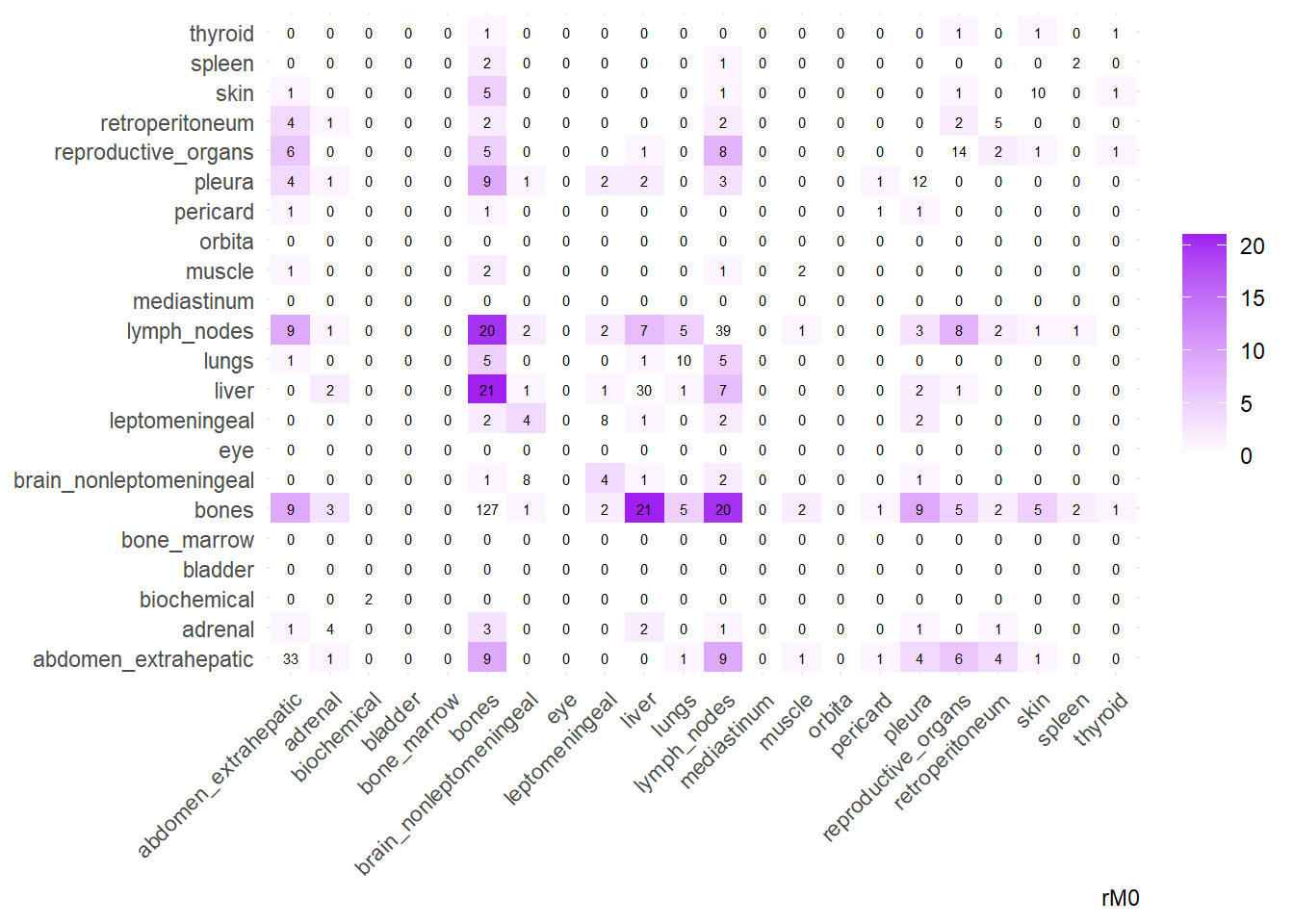
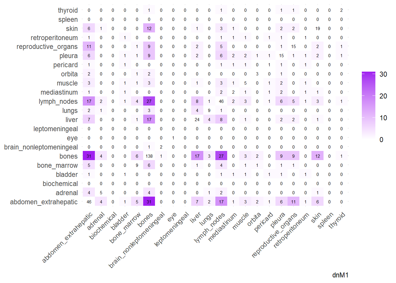
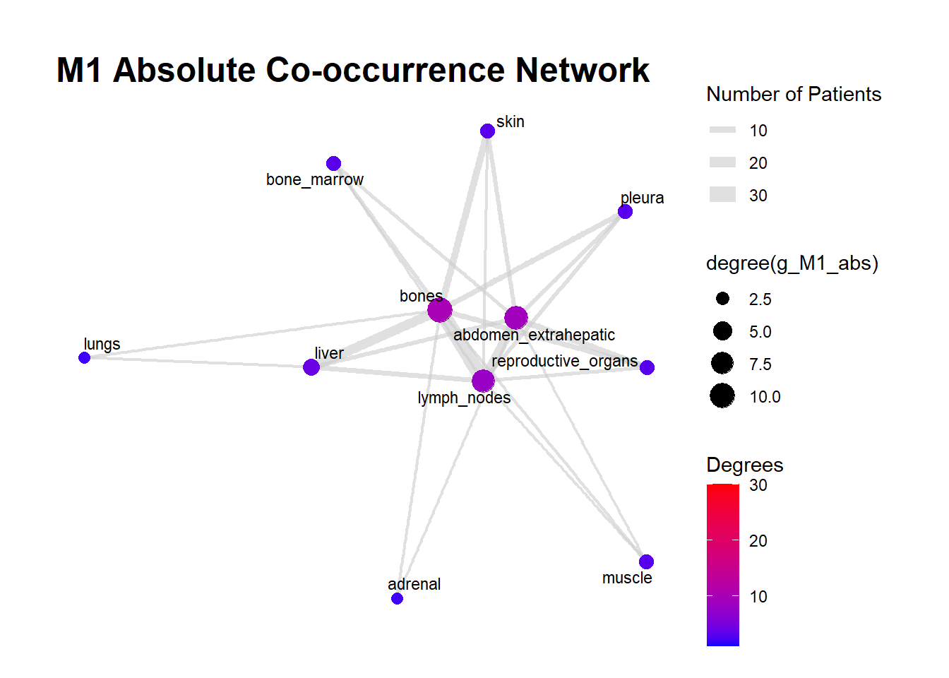
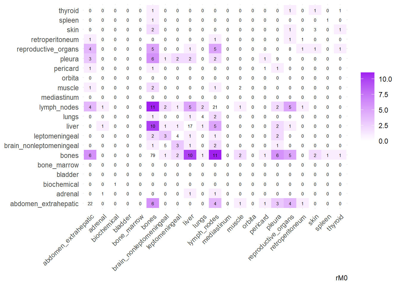
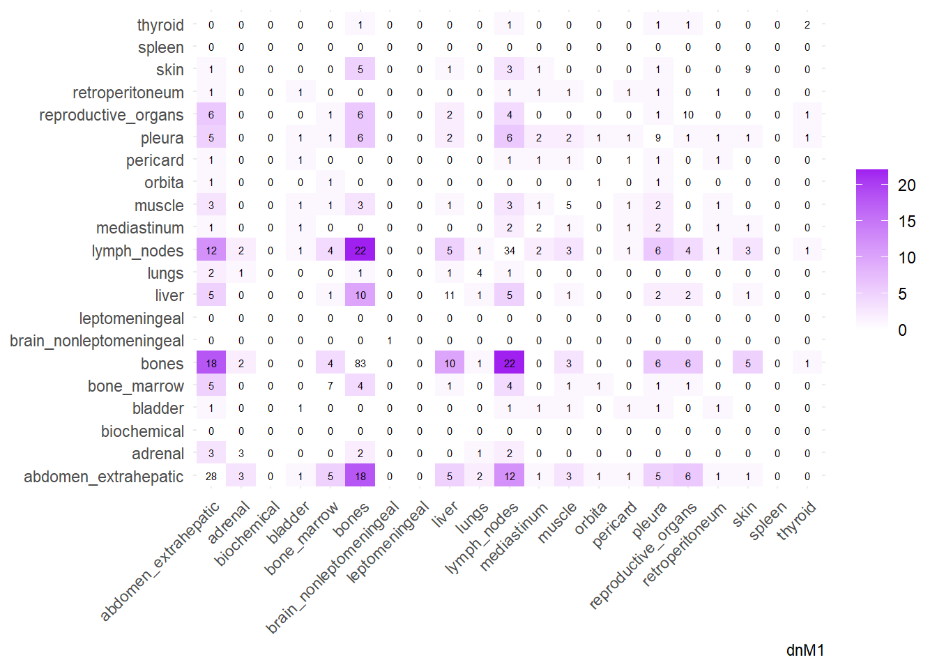
We can then operate on a co-occurrence matrix. This matrix displays the absolute frequency of the co-occurrence of metastases in two different sites, for each site-pair.
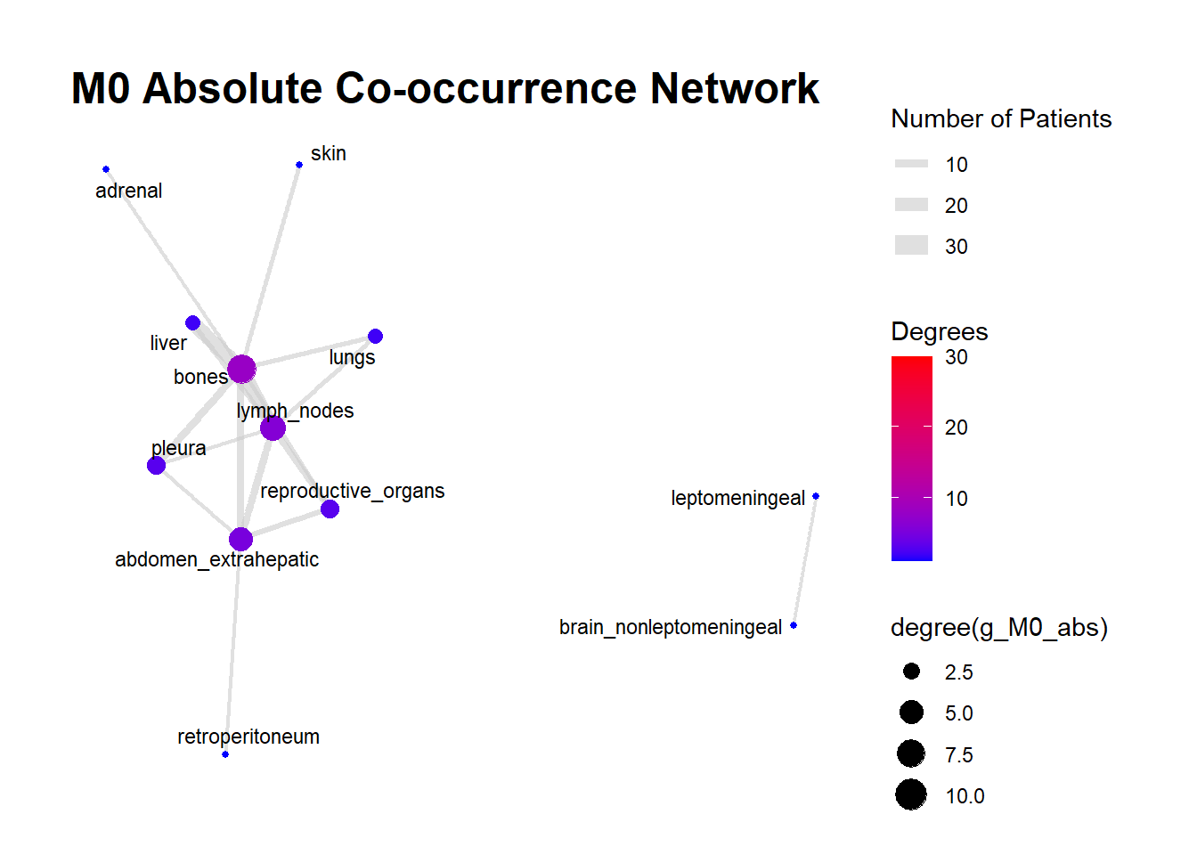
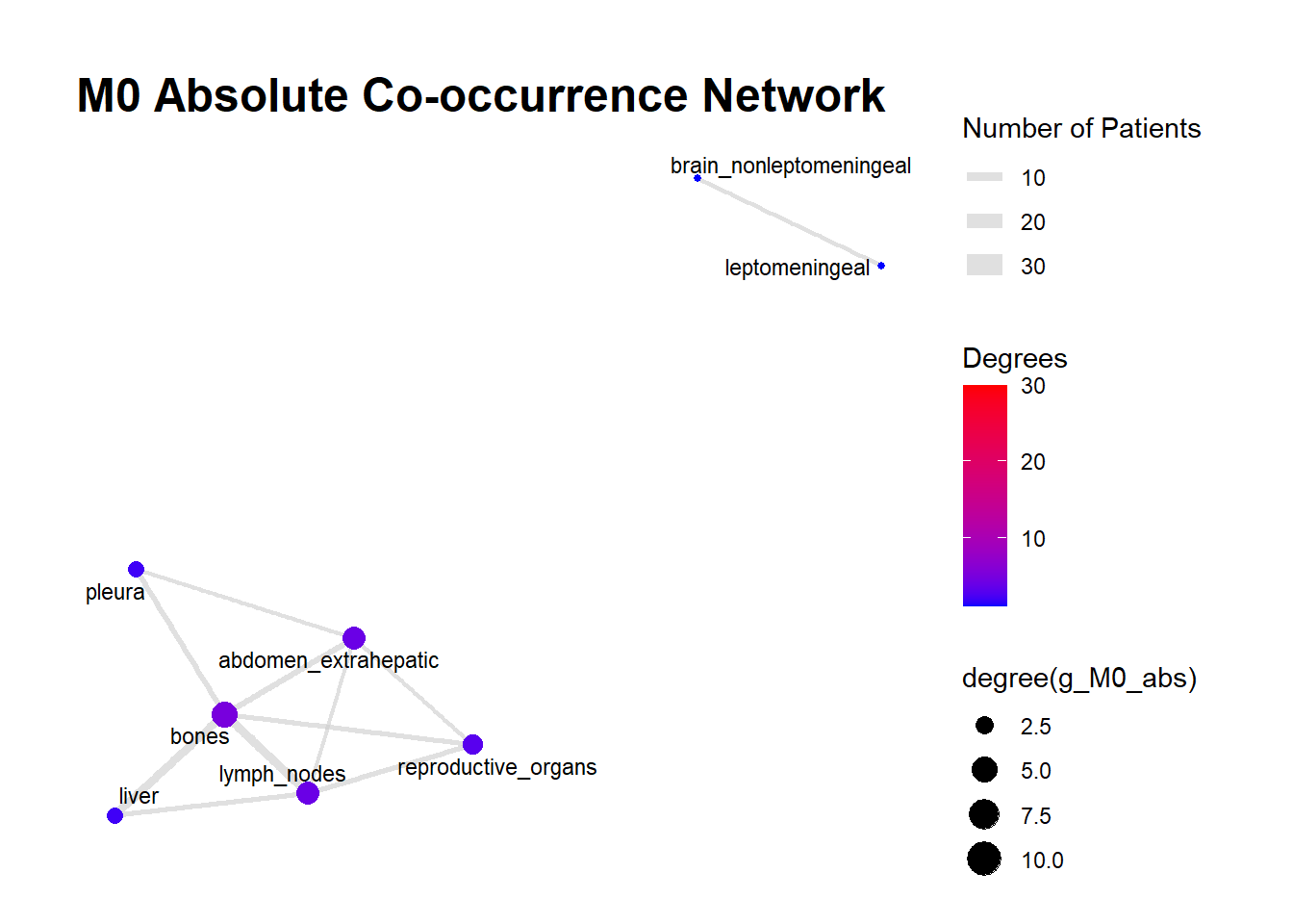
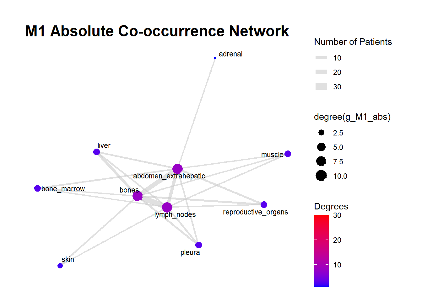
We can display these complex matrices with non-directed graphs. In this graph, each node is a site of metastasis, and each arrow represents a single co-occurrence. The more the site occur together, the wider is the arrow connecting the two nodes. Nodes that are more tightly connected (or part of the same “neighborhood”) tend to be grouped closer together. It minimizes edge crossing and tries to make edge lengths uniform, revealing clusters or central hubs in the network. The size represents the Degree of the node. This counts the number of unique connections a node has. A larger node means that entity co-occurs with a wider variety of other entities. A small node has fewer unique co-occurrences. The same holds true for the color of the nodes.
The most striking feature of the M0 network is its fragmentation. There is a distinct, isolated sub-network in the top left consisting of brain_nonleptomeningeal and leptomeningeal metastases. This indicates that in the recurrent setting, Central Nervous System (CNS) progression often occurs independently of the visceral metastatic burden. In contrast, the M1 network presents as a single, highly connected component. There are no isolated islands; every metastatic site is linked to the main cluster. This suggests that De Novo metastasis is a more systemic event where disease burden is correlated across all affected sites simultaneously.
The gray connecting lines (edges) in the M1 network appear thicker and more numerous compared to M0. This visualizes the results of your Jaccard analysis: sites in M1 are “co-occurring” more frequently and with stronger statistical association than in M0.
Bone_marrow and Muscle appear as distinct nodes in the M1 network but are absent or below the plotting threshold (3) in M0. The Retroperitoneum is visible in the visceral cluster of M0 but is not a labeled node in this view of M1, suggesting it may be a more specific site of failure in recurrent disease rather than a primary site in De Novo presentation.
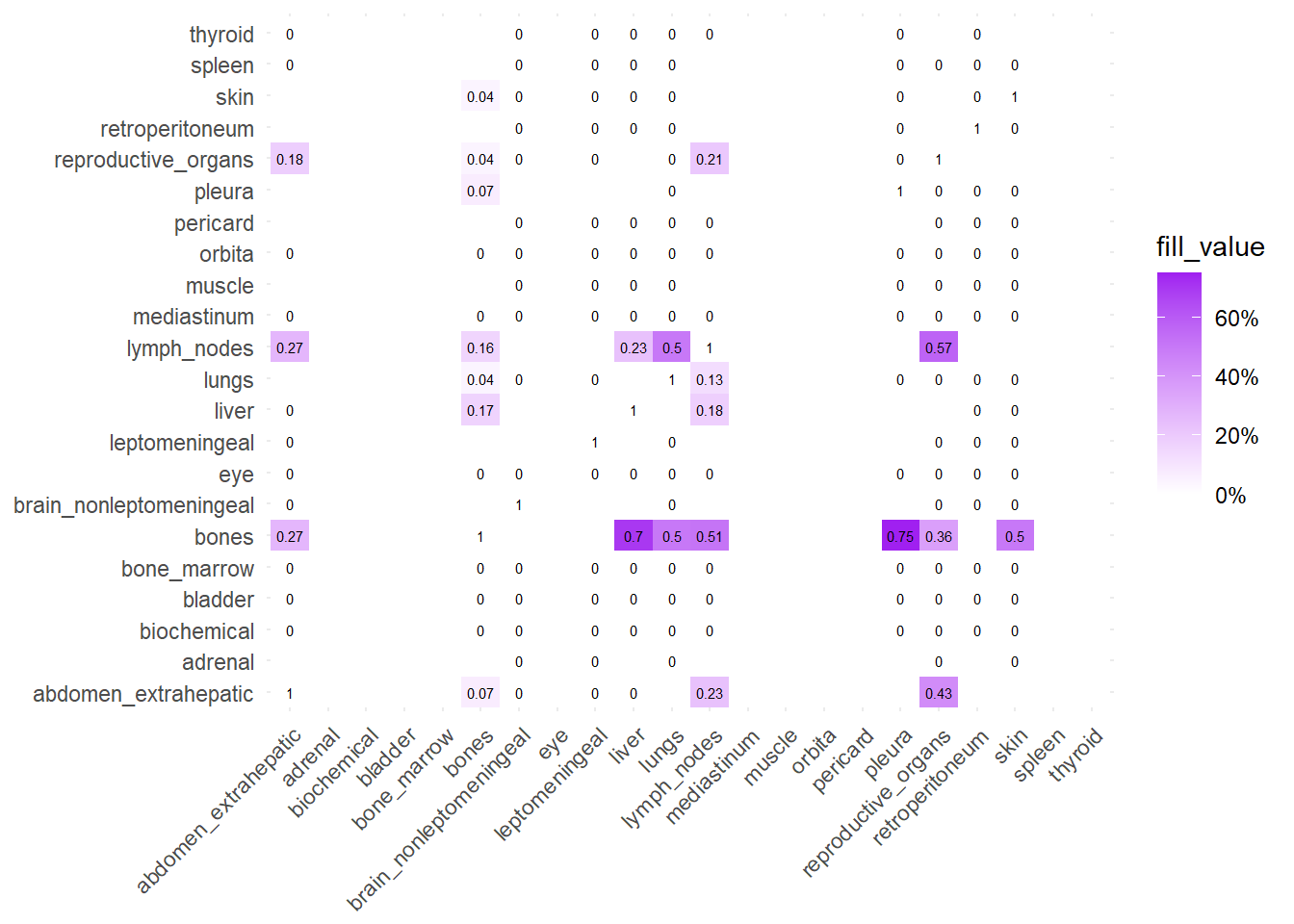
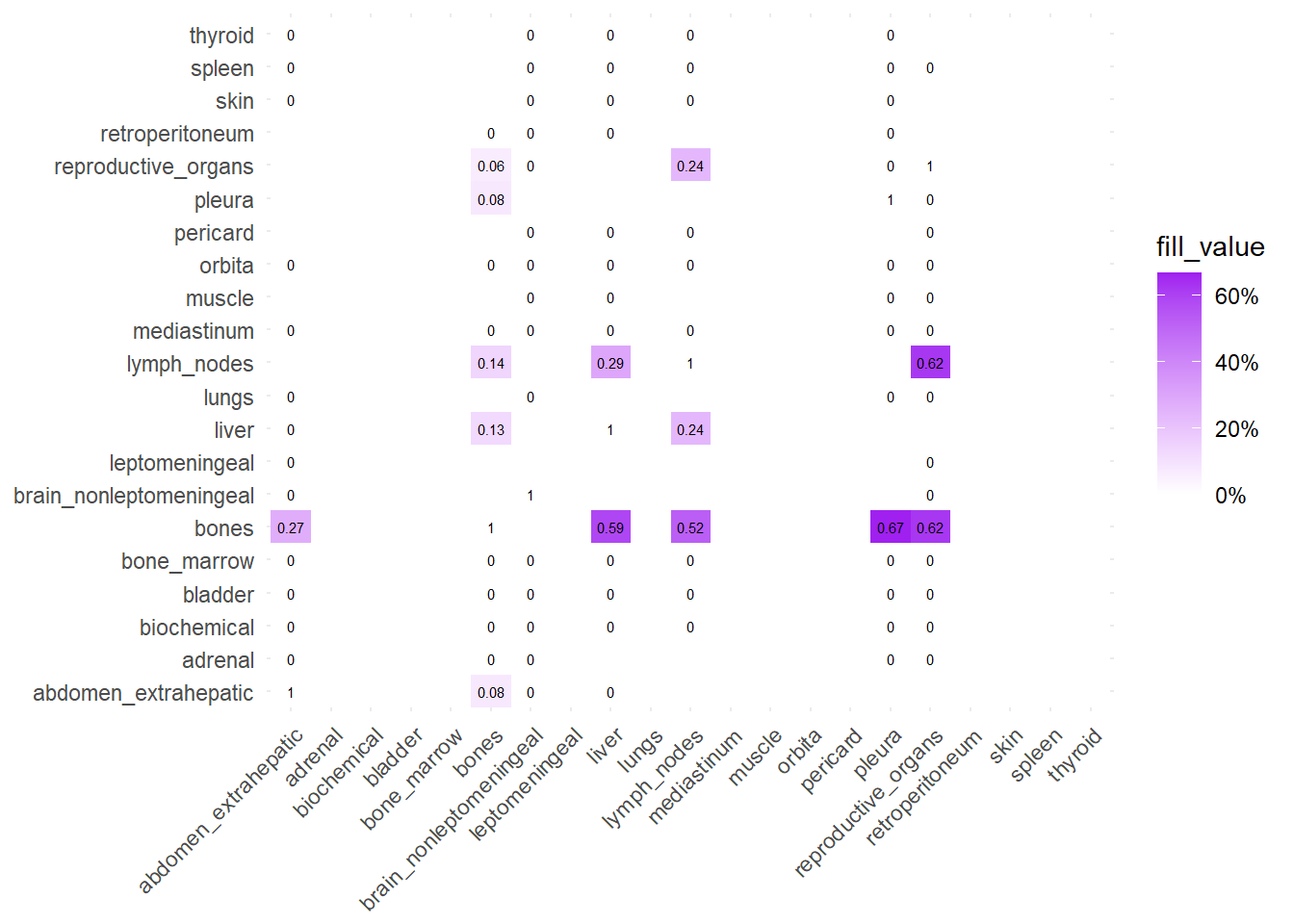
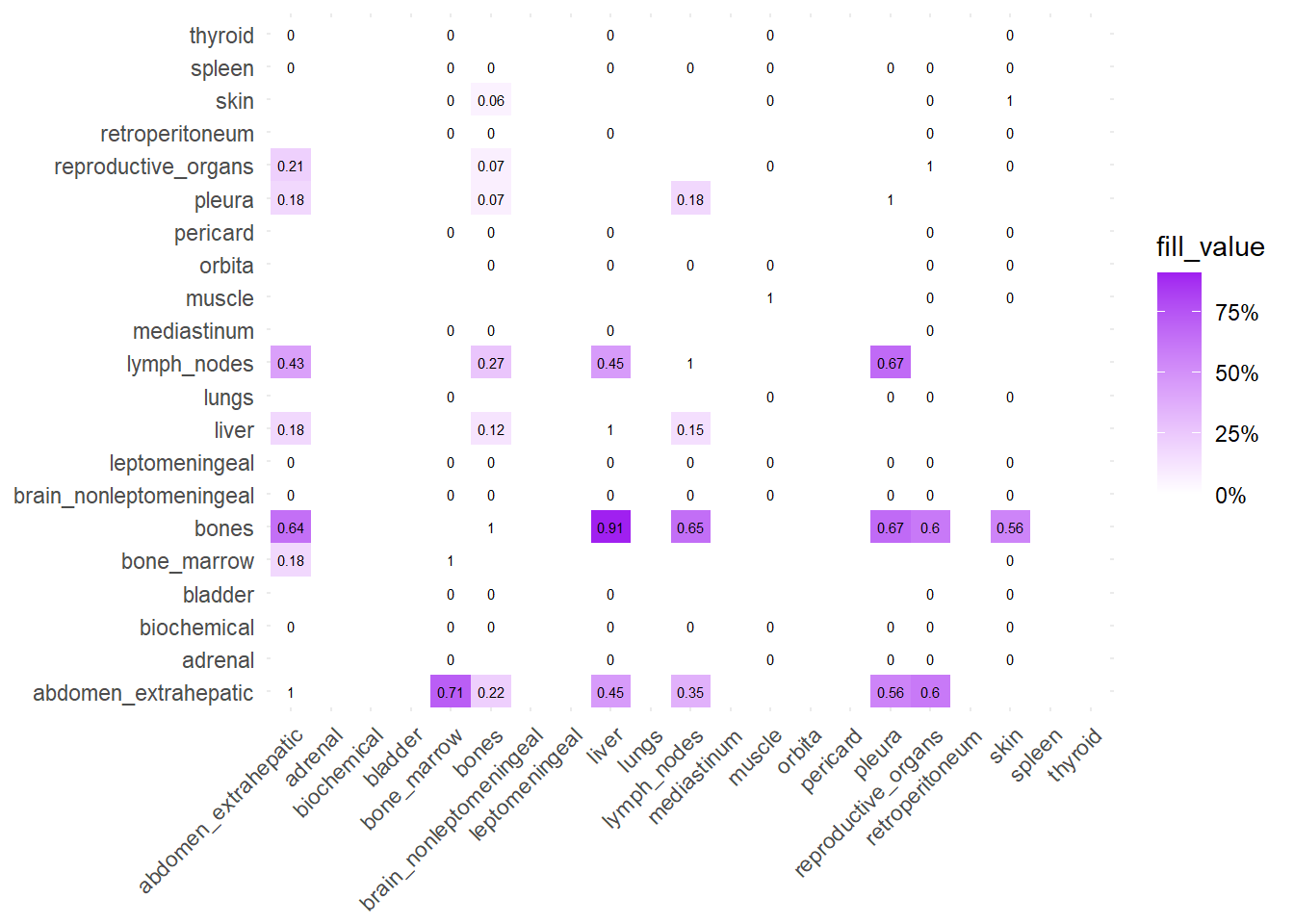
We can also compare the difference in the co-occurrence of metastases looking at the matrices of conditional probability or the matrix that report the contrasts between the two. Each cell of the matrix defines a conditional probability of occurrence: ‘conditional on having a metastasis on site A, what is the probability of having a metastasis also in site B?’. In the upper left triangle, the conditioning site are reported in the Y-axis. For the lower right triangle, the conditioning site are reported in the X-axis.
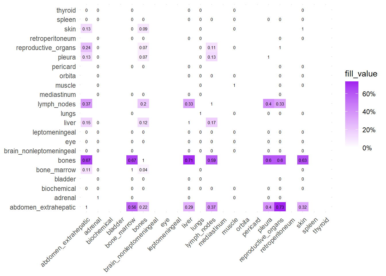
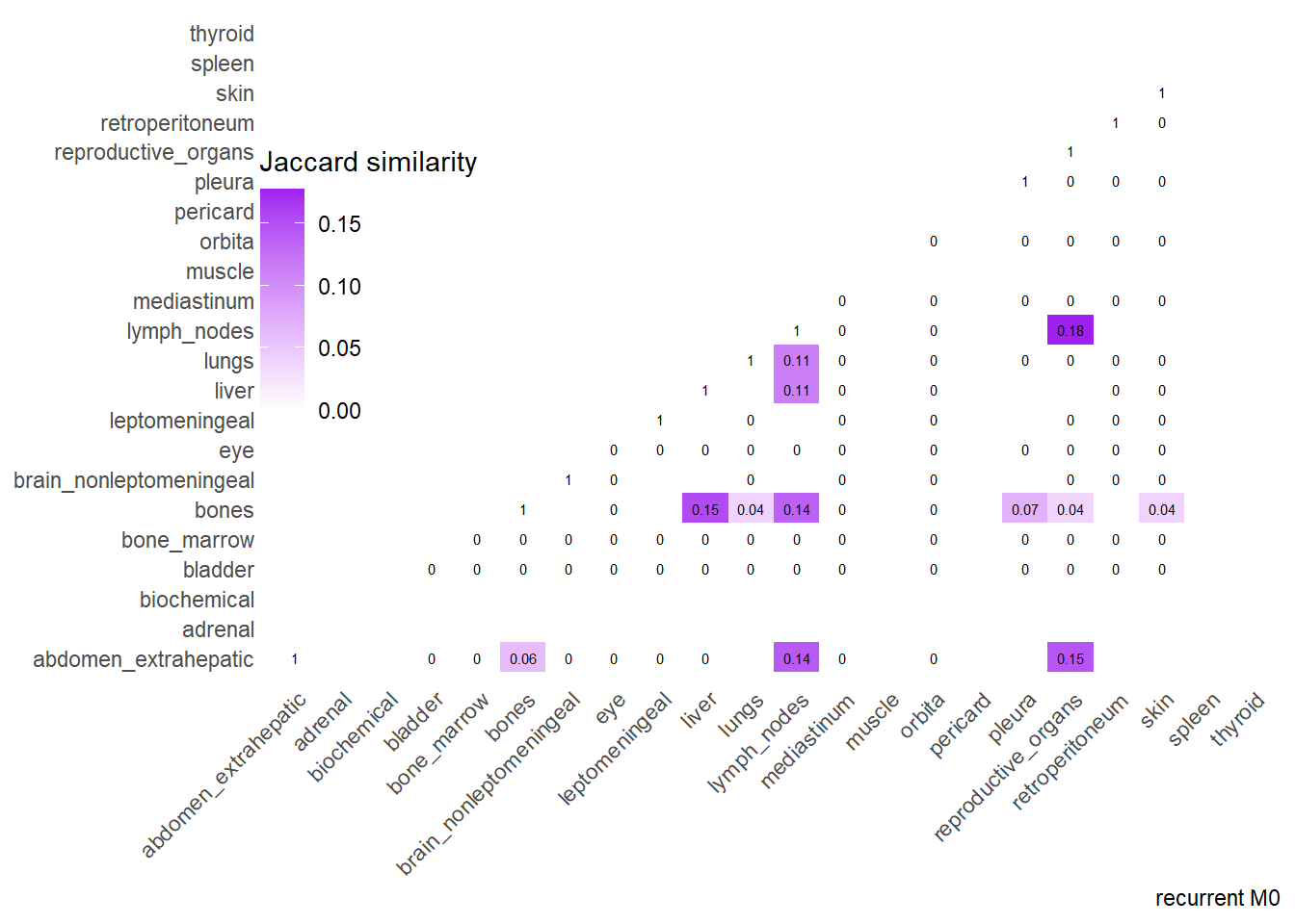
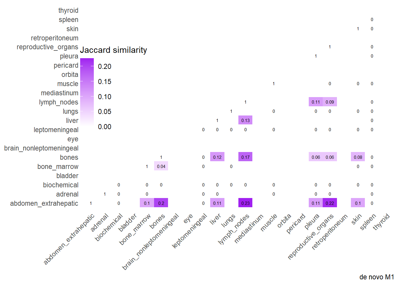
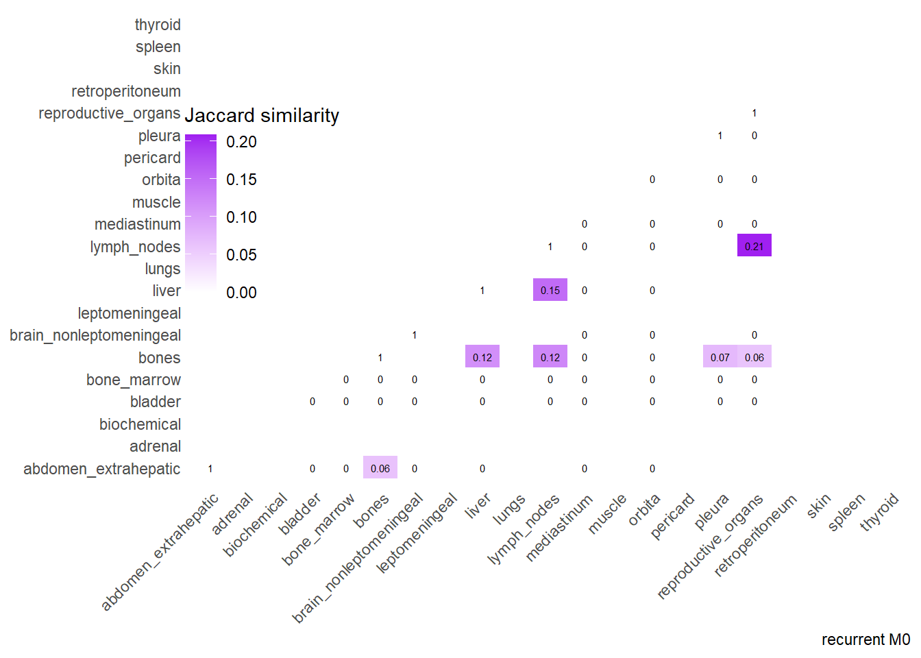
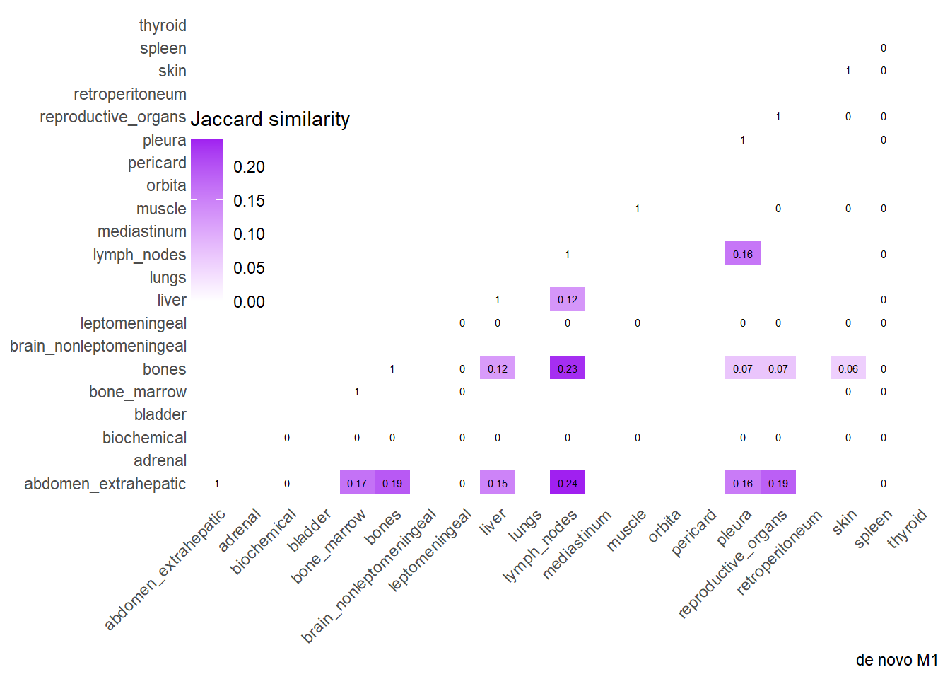
Finally, we can display the strenght of association by considering the jaccard index. I perform a comparative analysis of Jaccard Similarity between two conditions. It calculates how much “sites” overlap with one another in two different datasets, visualizes those overlaps, and finally plots the change in similarity between the two conditions.
The big matrices of co-occurrence are structured as follow: off-diagonals cells \((i, j)\) contain the count of the intersection (overlap) between site \(i\) and site \(j\). The Diagonal \((i, i)\) contains the total count for site \(i\) (since \(Intersection(A, A) = Total(A)\)). To get the Jaccard Index we compute \(J(A,B) = \frac{|A \cap B|}{|A \cup B|}\)
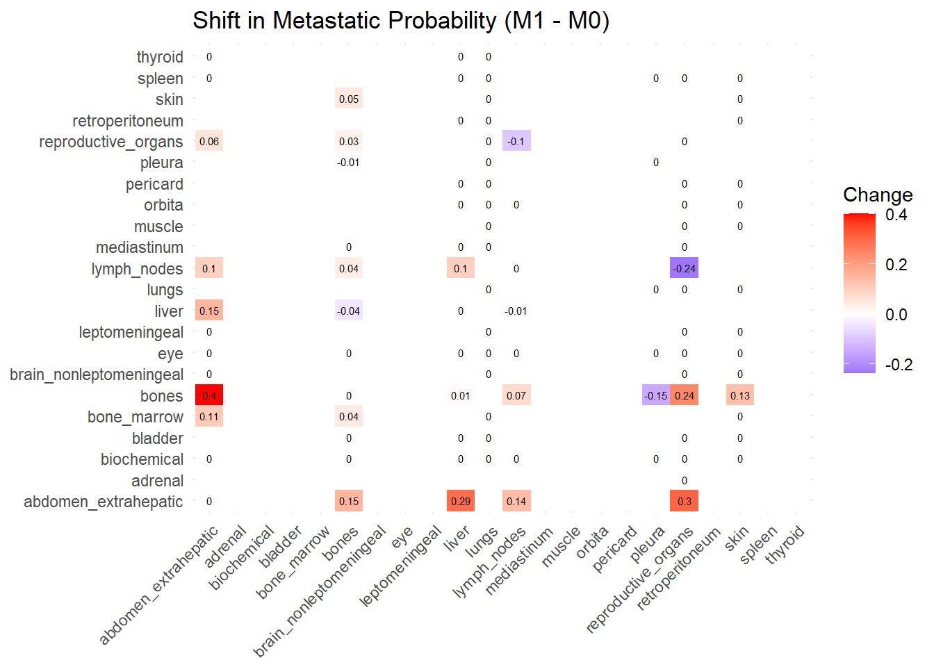
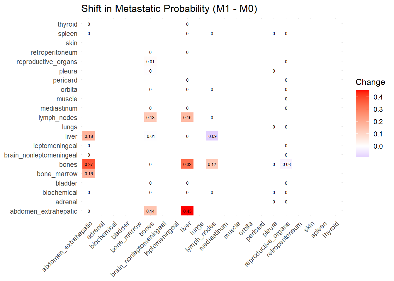
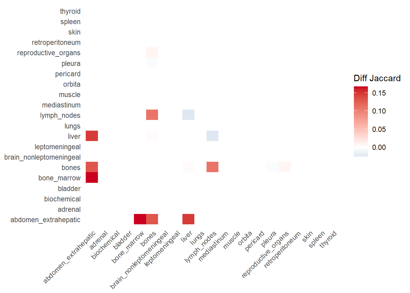
The following representations keep the lower triangle of the matrix to avoid duplicate visual information, remove the diagonal (self-similarity is always 1) and remove, values \(> 0.8\). This is likely done to increase contrast for lower/mid-range values, preventing the color scale from being “washed out” by perfect matches. In the graphs purple color means high similarity, whereas white low similarity. I then represent the difference in the jaccard similarities between M0 and M1. In the plot
Red (High/Positive): The value is positive, meaning similarity increased in M1 (sites are more alike).
Blue (Low/Negative): The value is negative, meaning similarity decreased in M1 (sites are diverging).
White: No change in similarity.

6.1 Multiple correspondence analysis
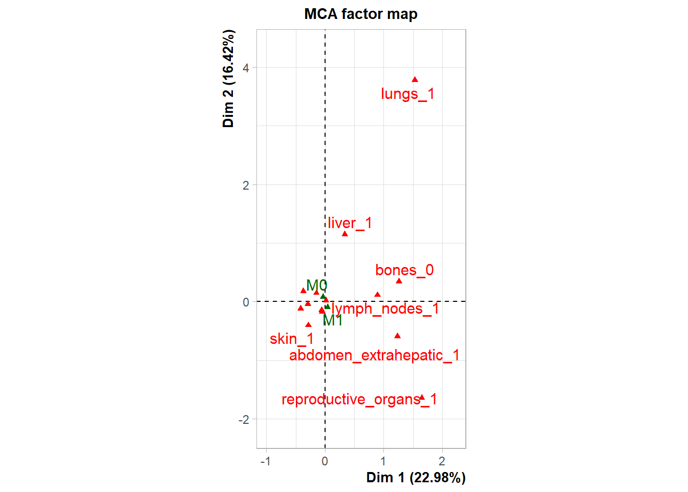
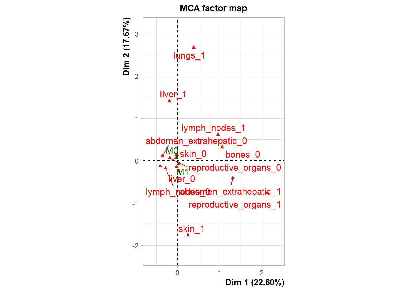
To move beyond pairwise associations and identify broader systemic patterns of metastasis, Multiple Correspondence Analysis (MCA) was performed on the binary presence/absence data of major metastatic sites (Skin, Reproductive Organs, Lymph Nodes, Lungs, Liver, Bones, Extrahepatic Abdomen).
Dimensionality Reduction: The multidimensional clinical data was reduced to principal components (dimensions) to visualize the underlying structure of the data.
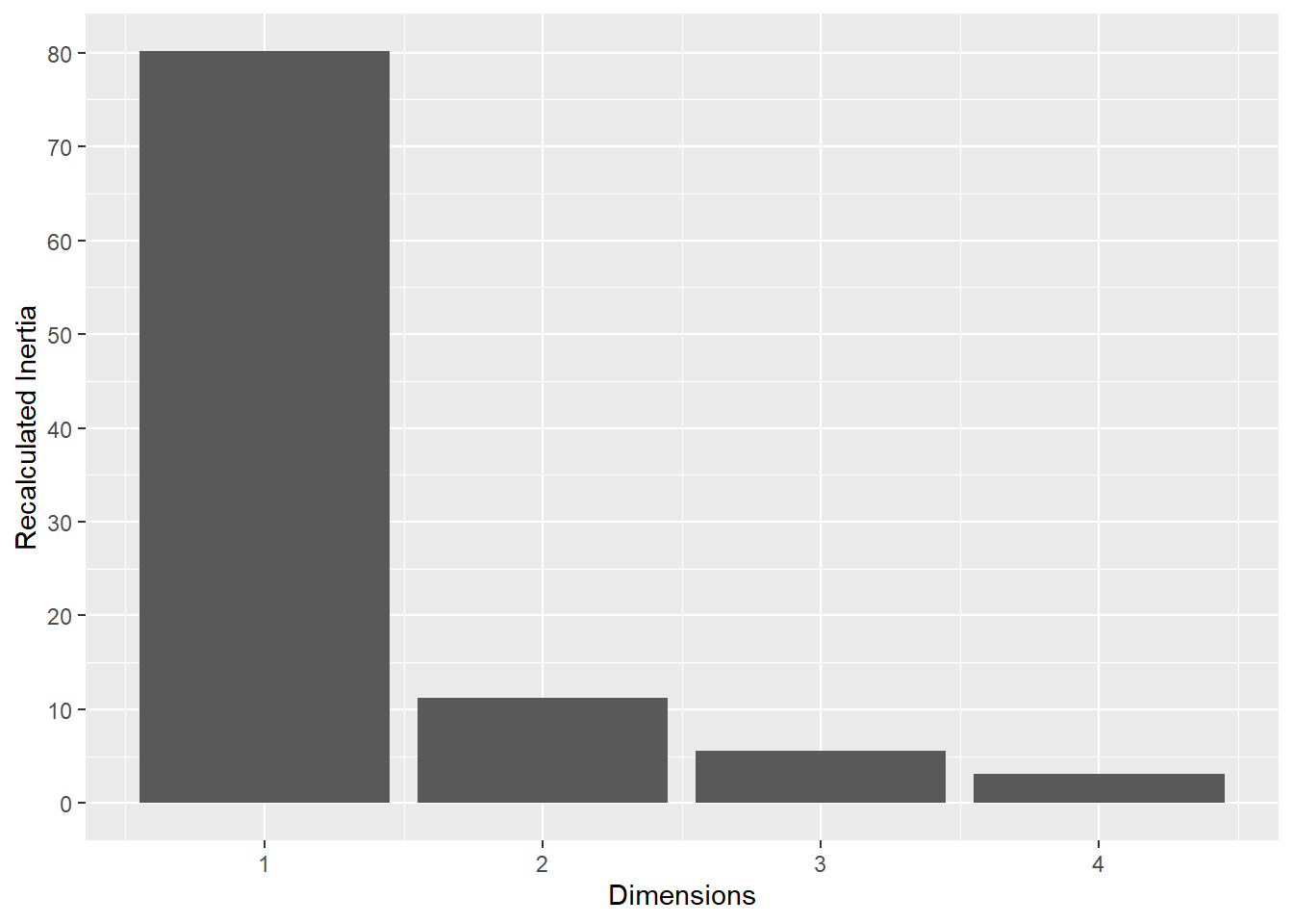
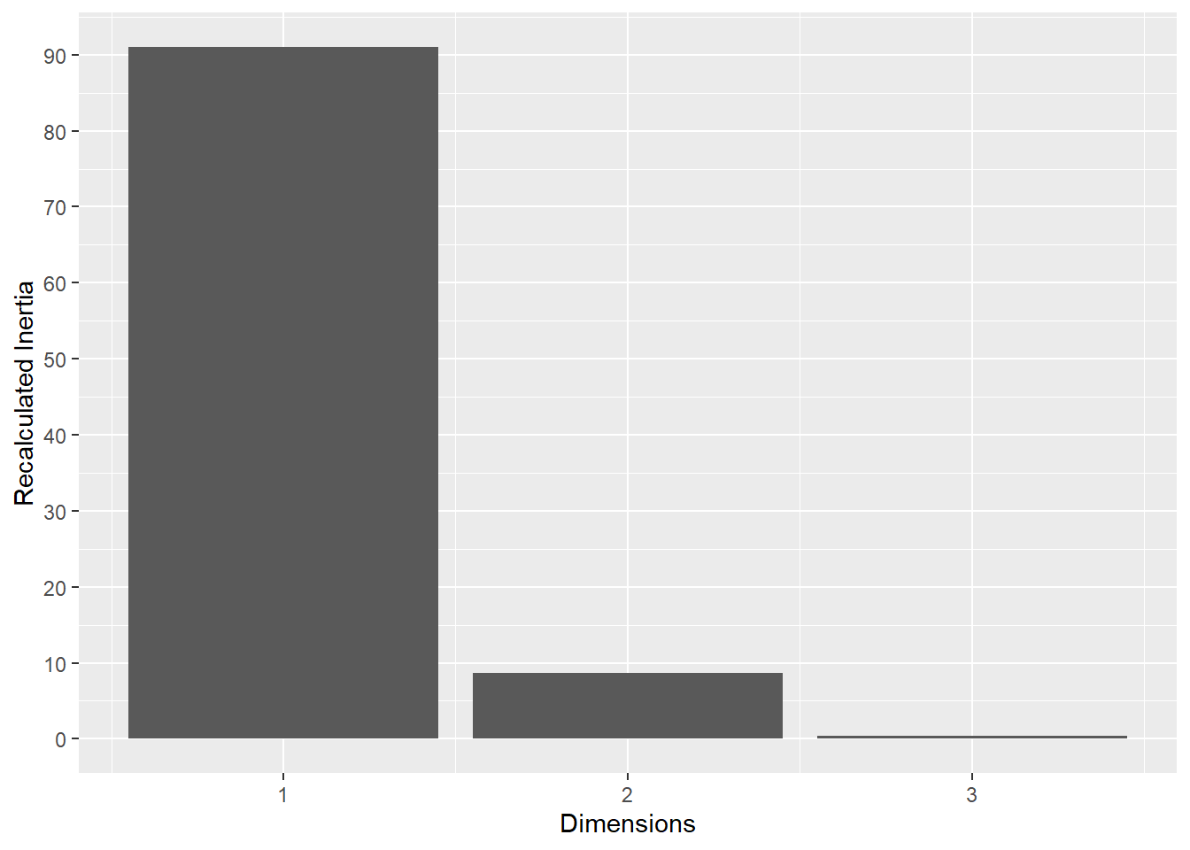
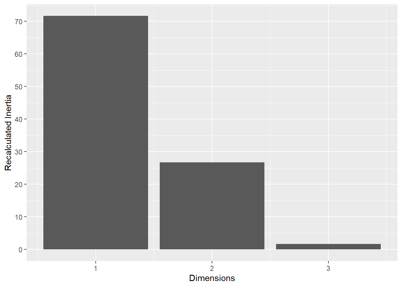
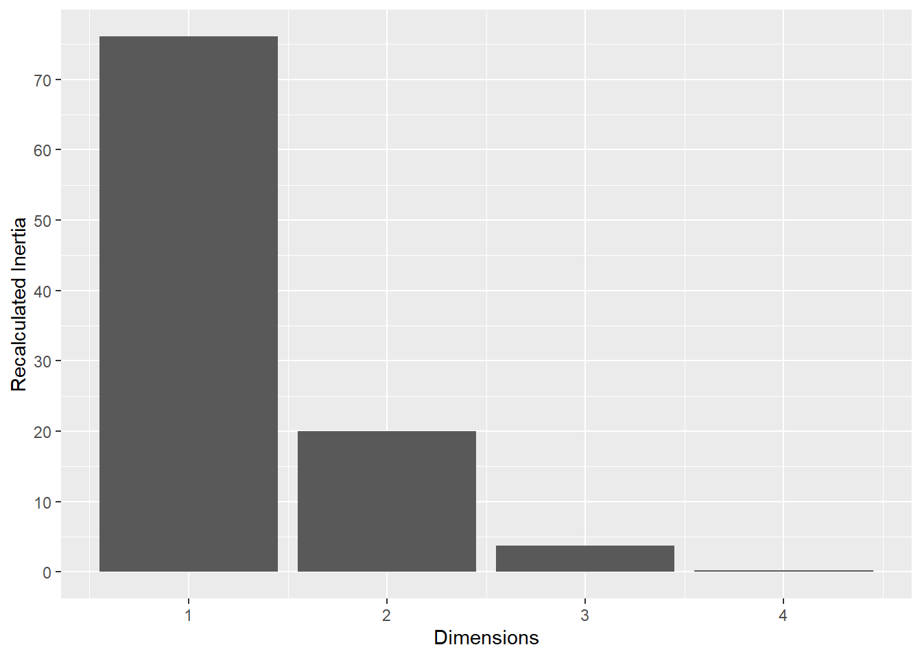
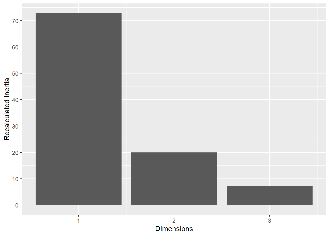
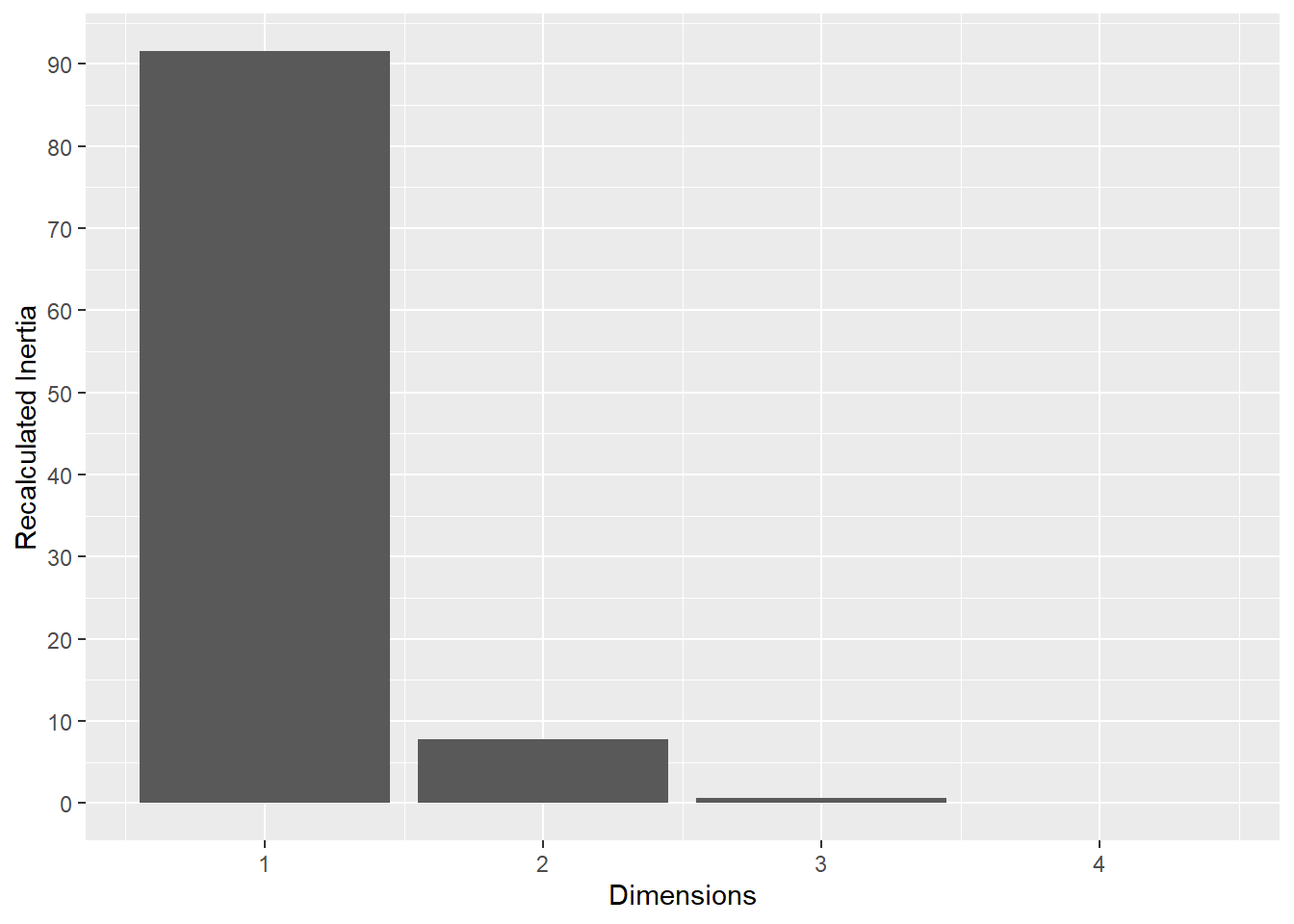
Inertia Correction: To address the characteristic inflation of noise in standard MCA, a Benzécri correction was applied to the raw eigenvalues. This yielded a recalibrated estimate of the explained variance (inertia) for each dimension, ensuring that only significant signals were interpreted.
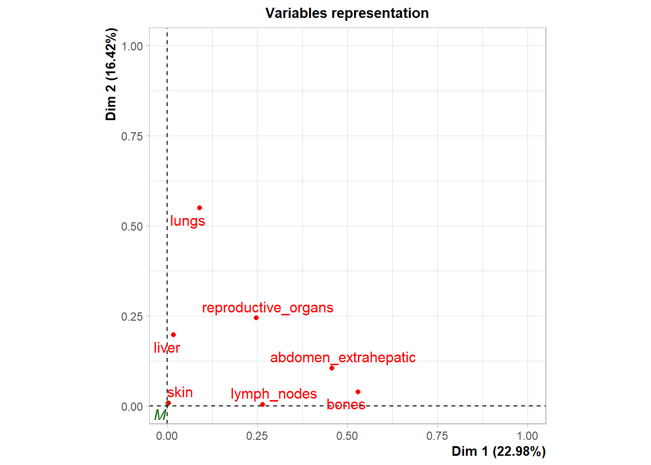
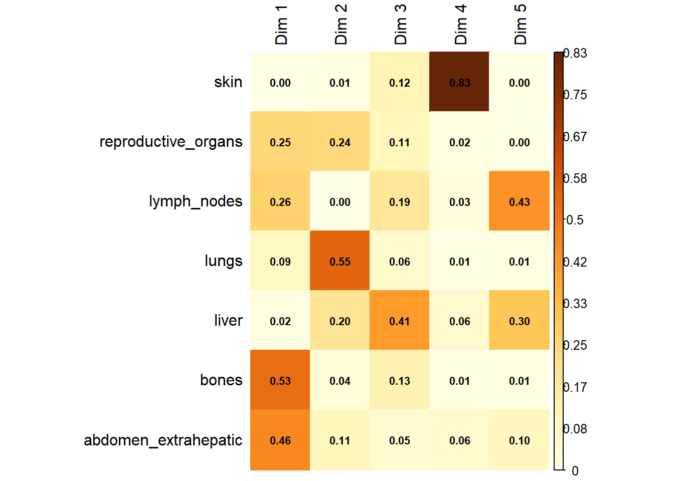
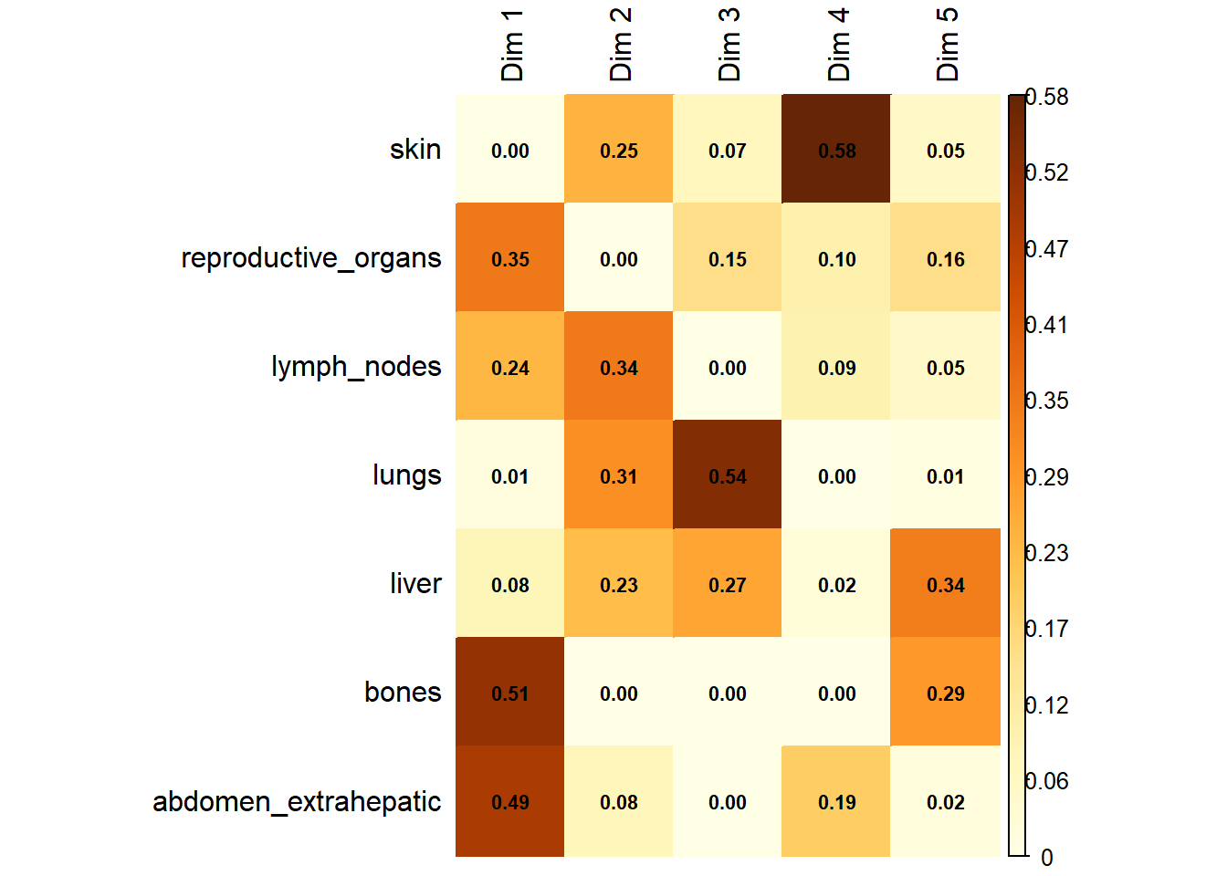
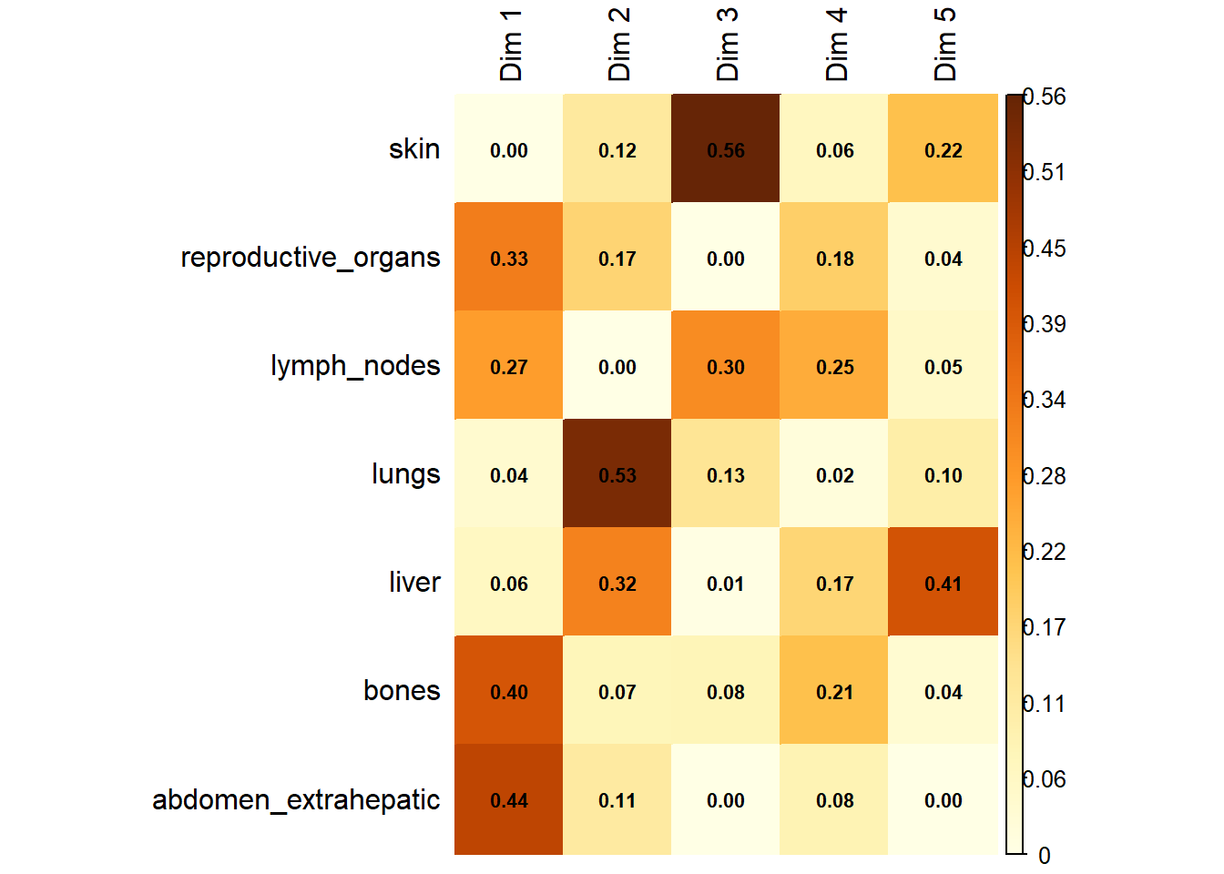
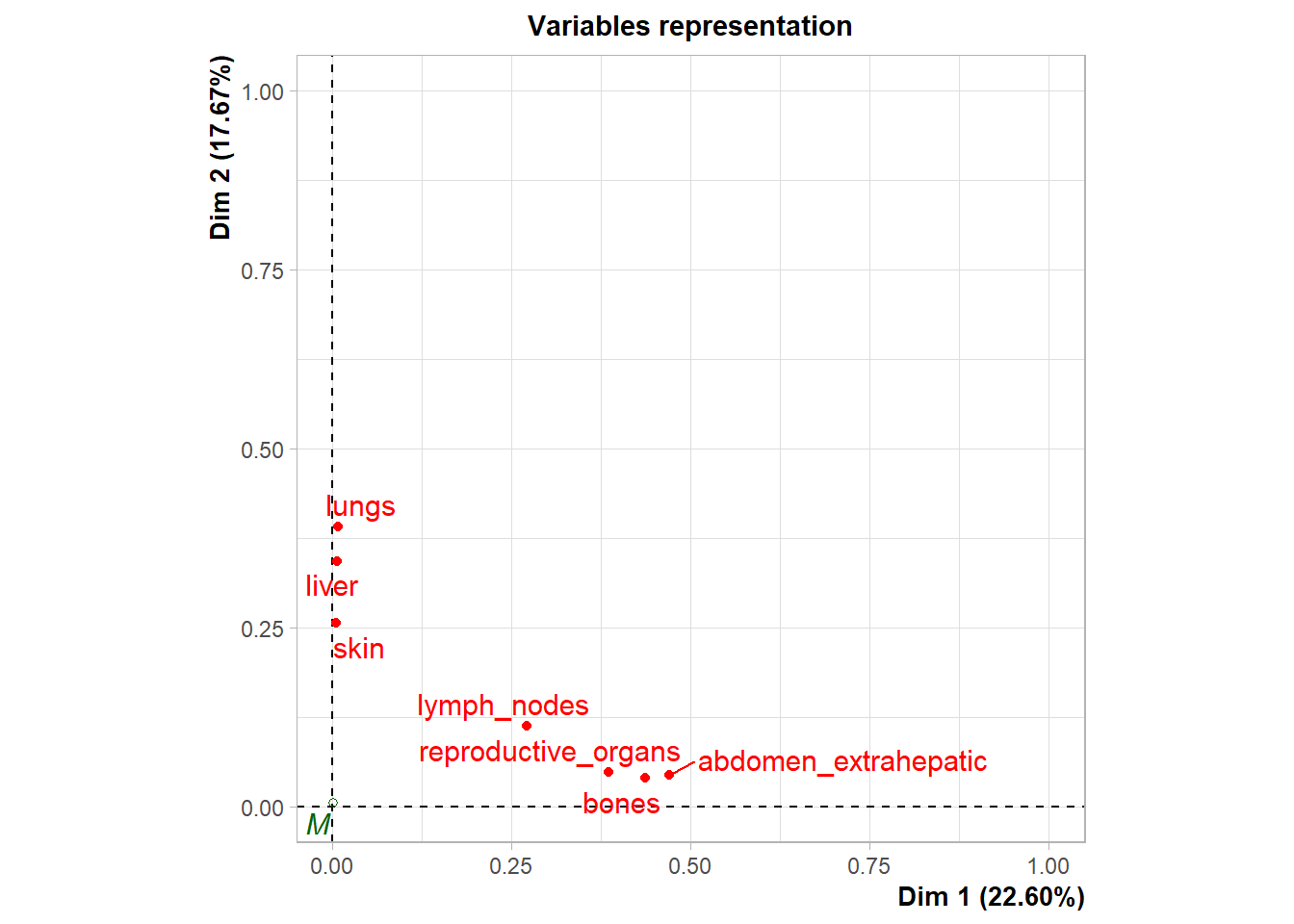
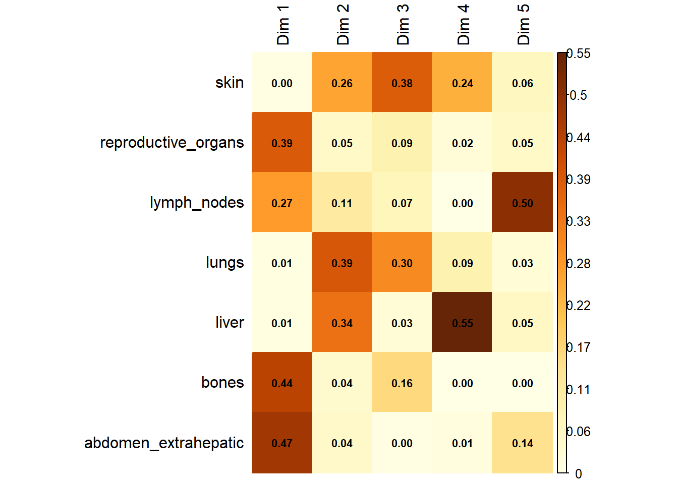
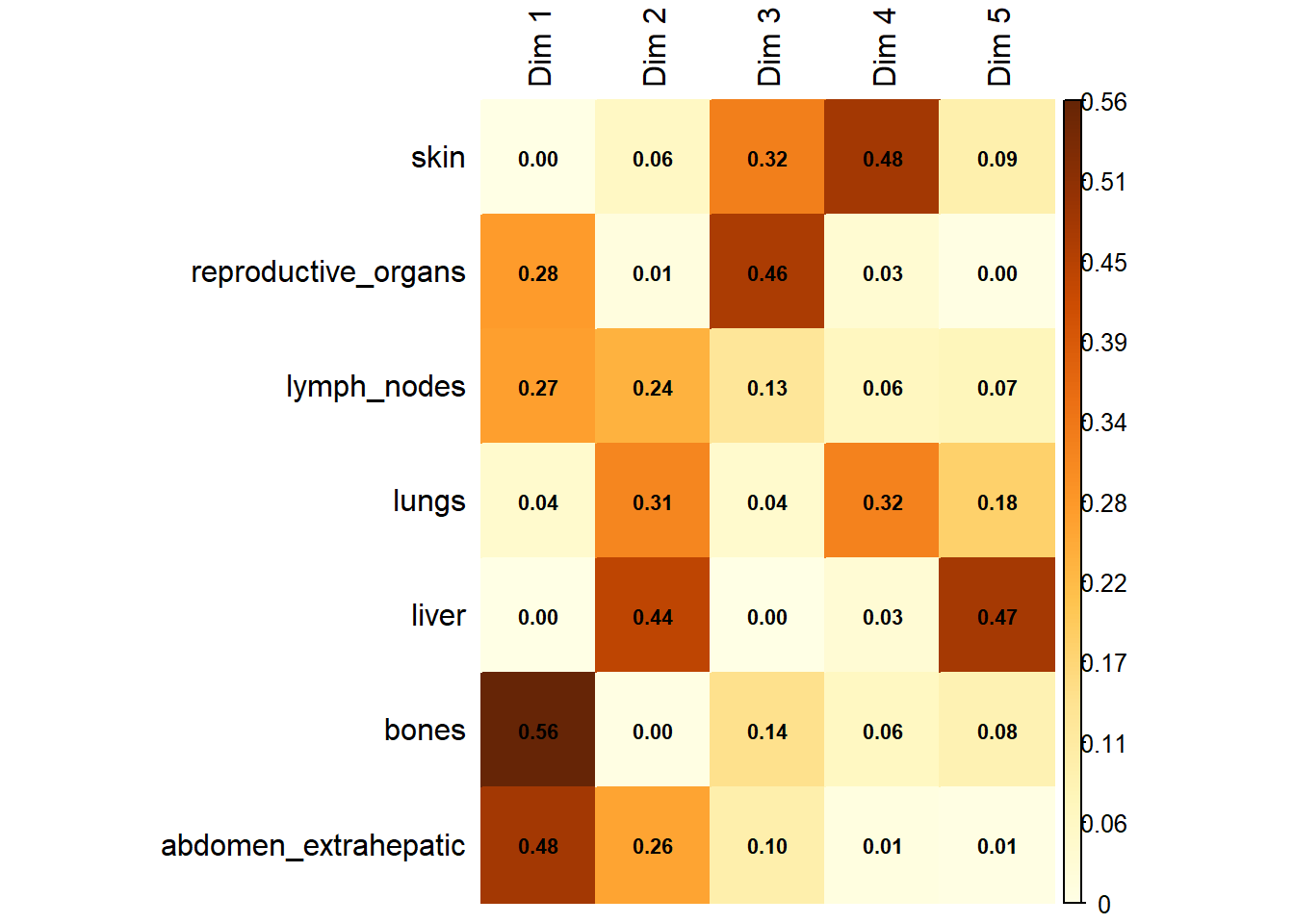
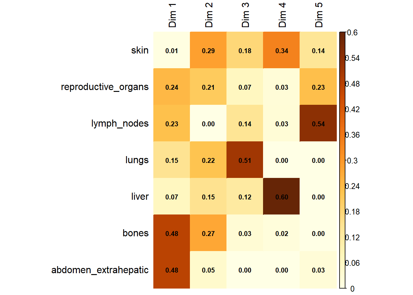
Variable Contribution: The association between specific metastatic sites and the resulting dimensions was assessed using the correlation ratio (\(\eta^2\)), identifying which organ sites were the primary drivers of variance in the dataset.
6.1.1 Patient Clustering (HCPC)
To classify patients into distinct clinical phenotypes based on their metastatic profiles:
Hierarchical Clustering: Hierarchical Clustering on Principal Components (HCPC) was applied to the coordinates derived from the MCA.
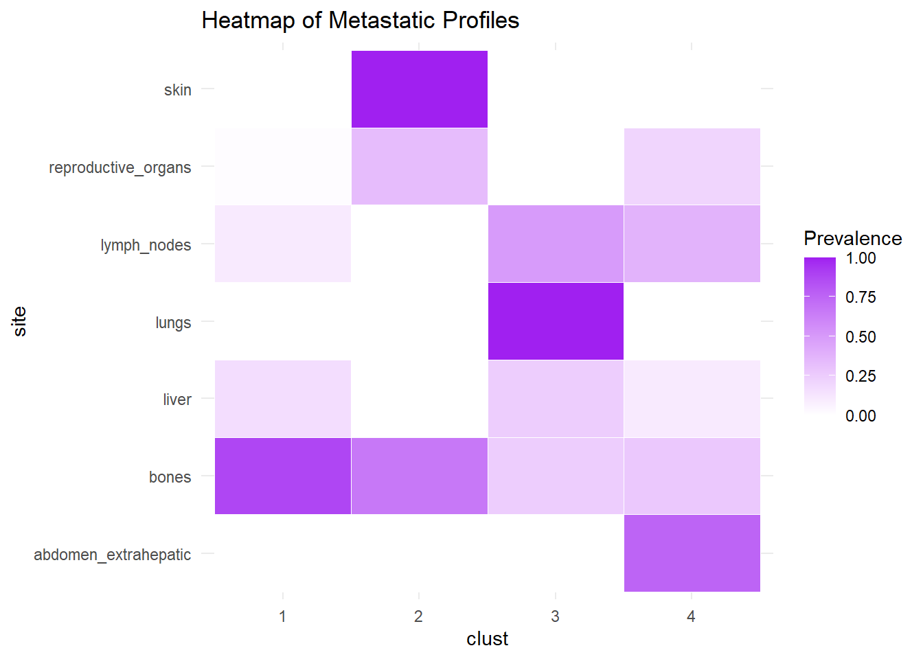
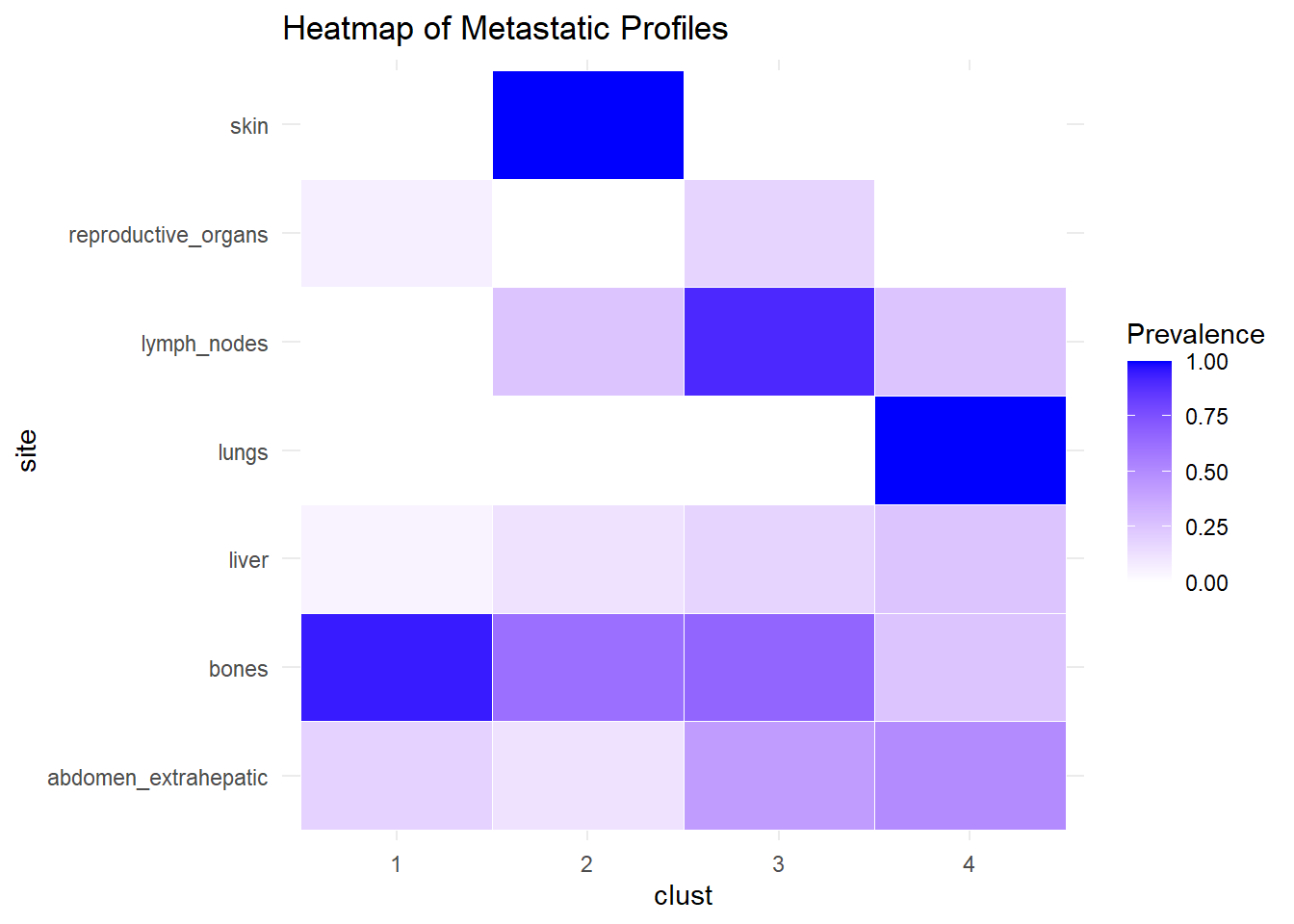
Subgroup Identification: The algorithm partitioned the patient population into four distinct clusters based on the similarity of their metastatic spread.
6.1.2 M0
This plot represents the percentage of variance explained by the first three dimension. The first dimension seems to explain the major part of the variance.
The following plot represents the correlation between the dimension and each site.
The following interactive plot represents the multidimensional space of the three prinicipal component to display the association between metastatic site.
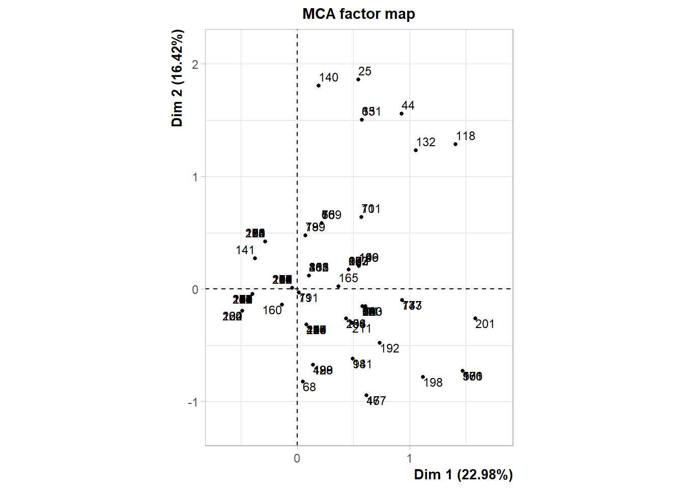
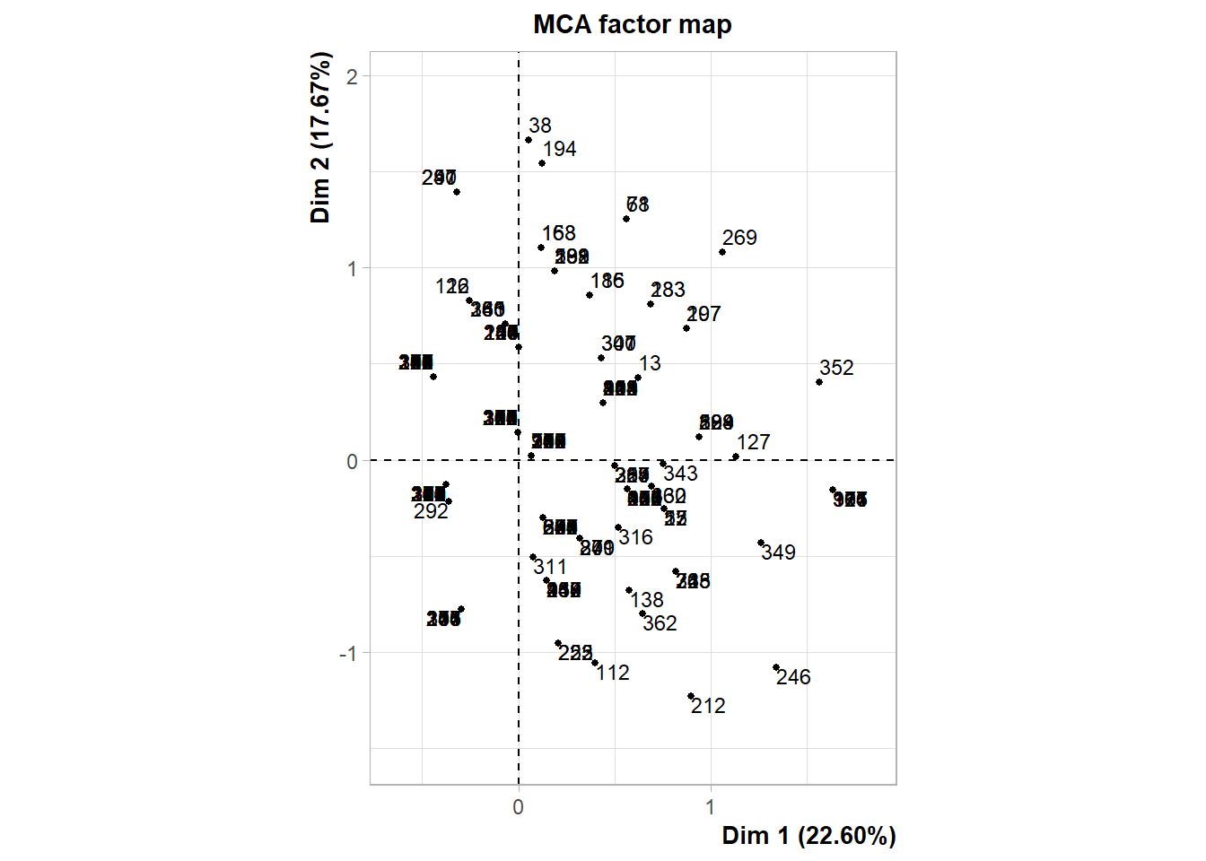
The following interactive plot represents the projection of the patients in the multi-dimensional space defined by the principal component. Patients are colored depending on the cluster identified.
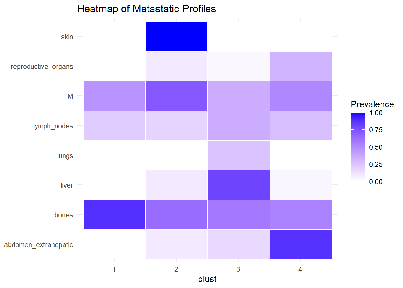
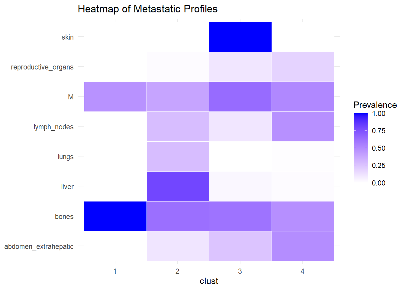
We describe the profiles identified considering the prevalence of each site within the cluster.
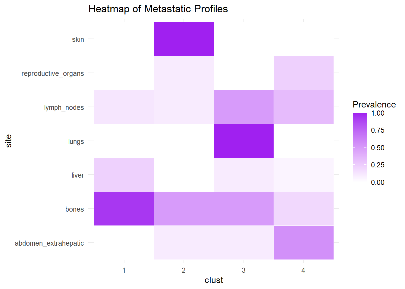
6.1.3 M1
The same analysis was performed for M1.
6.1.4 Merged
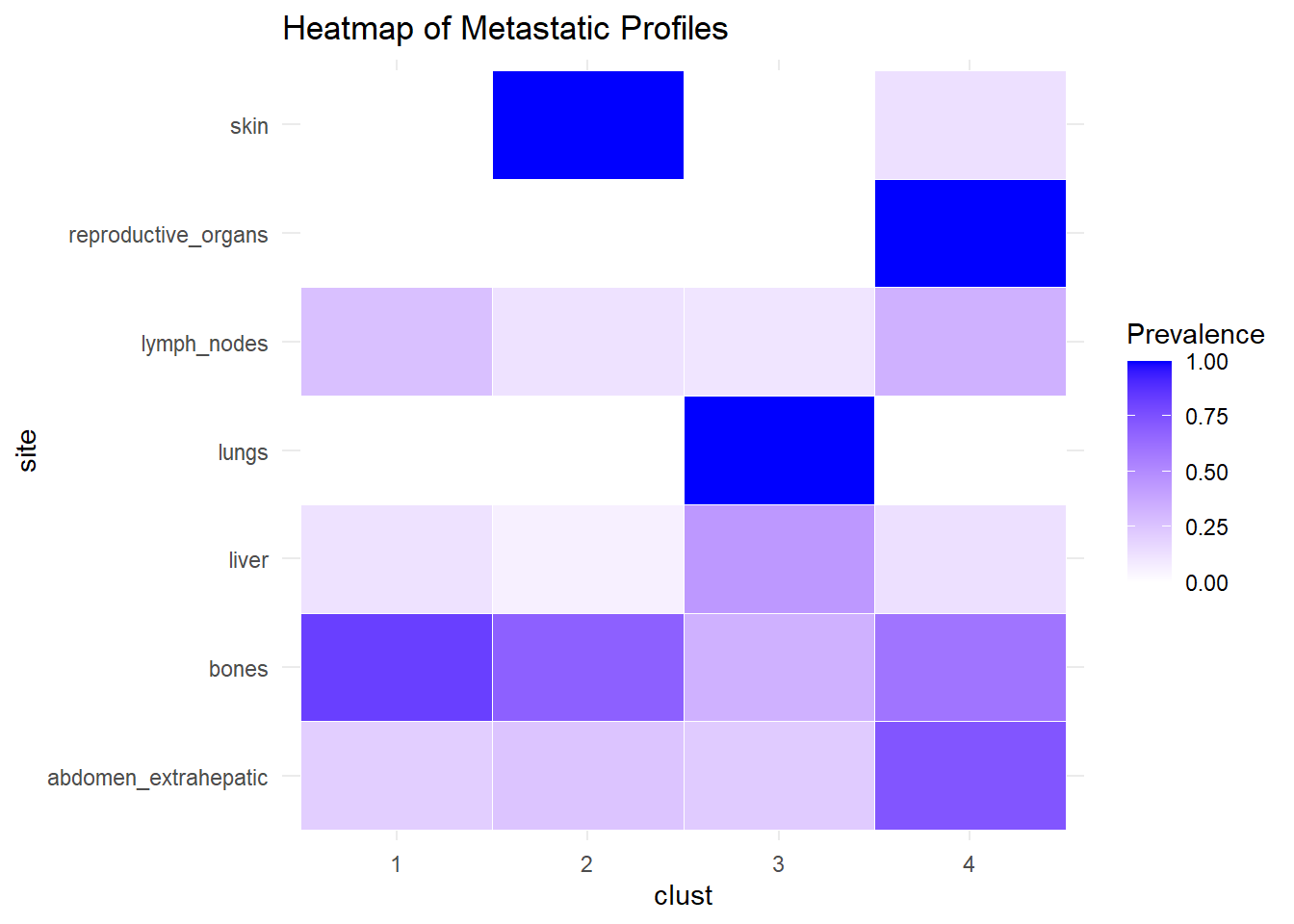
The following analysis was conducted with a merged matrix (M0 and M1). The association of M with the cluster identified has been described with the representation of the prevalence of the sites in the cluster. In this case, prevalence of M1 was computed to see whether specific clusters contain more M1. No differences were found.
6.2 Same analysis, but from 2015
6.2.1 Relative frequencies of site occurrence
| M0 (N=113) |
M1 (N=104) |
Overall (N=217) |
|
|---|---|---|---|
| Number of sites | |||
| 1 | 71 (62.8%) | 46 (44.2%) | 117 (53.9%) |
| 3 | 10 (8.8%) | 14 (13.5%) | 24 (11.1%) |
| 2 | 25 (22.1%) | 30 (28.8%) | 55 (25.3%) |
| 4 | 6 (5.3%) | 10 (9.6%) | 16 (7.4%) |
| 8 | 0 (0%) | 1 (1.0%) | 1 (0.5%) |
| 5 | 1 (0.9%) | 2 (1.9%) | 3 (1.4%) |
| 6 | 0 (0%) | 1 (1.0%) | 1 (0.5%) |
| bones | |||
| no | 34 (30.1%) | 21 (20.2%) | 55 (25.3%) |
| yes | 79 (69.9%) | 83 (79.8%) | 162 (74.7%) |
| abdomen_extrahepatic | |||
| no | 91 (80.5%) | 76 (73.1%) | 167 (77.0%) |
| yes | 22 (19.5%) | 28 (26.9%) | 50 (23.0%) |
| liver | |||
| no | 96 (85.0%) | 93 (89.4%) | 189 (87.1%) |
| yes | 17 (15.0%) | 11 (10.6%) | 28 (12.9%) |
| lymph_nodes | |||
| no | 92 (81.4%) | 70 (67.3%) | 162 (74.7%) |
| yes | 21 (18.6%) | 34 (32.7%) | 55 (25.3%) |
| pleura | |||
| no | 104 (92.0%) | 95 (91.3%) | 199 (91.7%) |
| yes | 9 (8.0%) | 9 (8.7%) | 18 (8.3%) |
| reproductive_organs | |||
| no | 105 (92.9%) | 94 (90.4%) | 199 (91.7%) |
| yes | 8 (7.1%) | 10 (9.6%) | 18 (8.3%) |
| brain_nonleptomeningeal | |||
| no | 108 (95.6%) | 103 (99.0%) | 211 (97.2%) |
| yes | 5 (4.4%) | 1 (1.0%) | 6 (2.8%) |
| leptomeningeal | |||
| no | 109 (96.5%) | 104 (100%) | 213 (98.2%) |
| yes | 4 (3.5%) | 0 (0%) | 4 (1.8%) |
| pericard | |||
| no | 112 (99.1%) | 103 (99.0%) | 215 (99.1%) |
| yes | 1 (0.9%) | 1 (1.0%) | 2 (0.9%) |
| lungs | |||
| no | 109 (96.5%) | 100 (96.2%) | 209 (96.3%) |
| yes | 4 (3.5%) | 4 (3.8%) | 8 (3.7%) |
| spleen | |||
| no | 112 (99.1%) | 104 (100%) | 216 (99.5%) |
| yes | 1 (0.9%) | 0 (0%) | 1 (0.5%) |
| muscle | |||
| no | 111 (98.2%) | 99 (95.2%) | 210 (96.8%) |
| yes | 2 (1.8%) | 5 (4.8%) | 7 (3.2%) |
| biochemical | |||
| no | 112 (99.1%) | 104 (100%) | 216 (99.5%) |
| yes | 1 (0.9%) | 0 (0%) | 1 (0.5%) |
| skin | |||
| no | 110 (97.3%) | 95 (91.3%) | 205 (94.5%) |
| yes | 3 (2.7%) | 9 (8.7%) | 12 (5.5%) |
| thyroid | |||
| no | 112 (99.1%) | 102 (98.1%) | 214 (98.6%) |
| yes | 1 (0.9%) | 2 (1.9%) | 3 (1.4%) |
| adrenal | |||
| no | 112 (99.1%) | 101 (97.1%) | 213 (98.2%) |
| yes | 1 (0.9%) | 3 (2.9%) | 4 (1.8%) |
| retroperitoneum | |||
| no | 112 (99.1%) | 103 (99.0%) | 215 (99.1%) |
| yes | 1 (0.9%) | 1 (1.0%) | 2 (0.9%) |
| bone_marrow | |||
| no | 113 (100%) | 97 (93.3%) | 210 (96.8%) |
| yes | 0 (0%) | 7 (6.7%) | 7 (3.2%) |
| orbita | |||
| no | 113 (100%) | 103 (99.0%) | 216 (99.5%) |
| yes | 0 (0%) | 1 (1.0%) | 1 (0.5%) |
| bladder | |||
| no | 113 (100%) | 103 (99.0%) | 216 (99.5%) |
| yes | 0 (0%) | 1 (1.0%) | 1 (0.5%) |
| mediastinum | |||
| no | 113 (100%) | 102 (98.1%) | 215 (99.1%) |
| yes | 0 (0%) | 2 (1.9%) | 2 (0.9%) |
6.3 Multiple correspondence analysis
6.3.1 M0
6.3.2 M1
6.3.3 Merged